The mistake comes when it is elevated from a heuristic to a principle.

Gary Smith pointed me to this post, “Don’t worship math: Numbers don’t equal insight,” subtitled, “The unwarranted assumption that investing in stocks is like rolling dice has led to some erroneous conclusions and extraordinarily conservative advice,” which reminded me of my discussion with Nate Silver a few years ago regarding his mistaken claim that, “the most robust assumption is usually that polling is essentially a random walk, i.e., that the polls are about equally likely to move toward one or another candidate, regardless of which way they have moved in the past.” My post was called, “Politics is not a random walk: Momentum and mean reversion in polling,” and David Park, Noah Kaplan, and I later expanded that into a paper, “Understanding persuasion and activation in presidential campaigns: The random walk and mean-reversion models.”

The random walk model for polls is a bit like the idea that the hot hand is a fallacy: it’s an appealing argument that has a lot of truth to it (as compared to the alternative model that poll movement or sports performance is easily predictable given past data) but is not quite correct, and the mistake comes when it is elevated from a heuristic to a principle.

This mistake happens a lot, no? It comes up in statistics all the time.

P.S. Some discussion in comments on stock market and investing. I know nothing about that topic; the above post is just about the general problem of people elevating a heuristic to a principle.

“The market can become rational faster than you can get out”

Palko pointed me to one of these stories about a fraudulent online business that crashed and burned. I replied that it sounded a lot like Theranos. The conversation continued:

Palko: Sounds like all the unicorns. The venture capital model breeds these things.

Me: Unicorns aren’t real, right?

Palko: Unicorns are mythical beasts and those who invest in them are boobies.

Me: Something something longer than something something stay solvent.

Palko: That’s good advice for short sellers, but it’s good to remember the corollary: the market can become rational faster than you can get out.

Good point.

Straining on the gnat of the prior distribution while swallowing the camel that is the likelihood. (Econometrics edition)

Jason Hawkins writes:

I recently read an article by the econometrician William Greene of NYU and others (in a 2005 book). They state the following:

The key difference between Bayesian and classical approaches is that Bayesians treat the nature of the randomness differently. In the classical view, the randomness is part of the model; it is the heterogeneity of the taste parameters, across individuals. In the Bayesian approach, the randomness ‘represents’ the uncertainty in the mind of the analyst (conjugate priors notwithstanding). Therefore, from the classical viewpoint, there is a ‘true’ distribution of the parameters across individuals. From the Bayesian viewpoint, in principle, there could be two analysts with different, both legitimate, but substantially different priors, who therefore could obtain very different, albeit both legitimate, posteriors.

My understanding is that this statement runs counter to the Berstein-von Mises theorem, which in the wording of Wikipedia “ assumes there is some true probabilistic process that generates the observations, as in frequentism” (my emphasis). Their context is comparing individual parameters from a mixture model, which can be taken from the posterior of a Bayesian inference or (in the frequentist case) obtained through simulation. I was particularly struck by their terming randomness as part of the model in the frequentist approach, which to me reads more as a feature of Bayesian approaches that are driven by uncertainty quantification.

My reply: Yes, I disagree with the above-quoted passage. They are exhibiting a common misunderstanding. I’ll respond with two points:

1. From the Bayesian perspective there also is a true parameter; see for example Appendix B of BDA for a review of the standard asymptotic theory. That relates to Hawkins’s point about the Berstein-von Mises theorem.

2. Greene et al. write, “From the Bayesian viewpoint, in principle, there could be two analysts with different, both legitimate, but substantially different priors, who therefore could obtain very different, albeit both legitimate, posteriors.” The same is true in the classical viewpoint; just replace the word “priors” by “likelihoods” or, more correctly, “data models.” Hire two different econometricians to fit two different models to your data and they can get “very different, albeit both legitimate” inferences.

Hawkins sends another excerpts from the paper:

The Bayesian approach requires the a priori specification of prior distributions for all of the model parameters. In cases where this prior is summarising the results of previous empirical research, specifying the prior distribution is a useful exercise for quantifying previous knowledge (such as the alternative currently chosen). In most circumstances, however, the prior distribution cannot be fully based on previous empirical work. The resulting specification of prior distributions based on the analyst’s subjective beliefs is the most controversial part of Bayesian methodology. Poirier (1988) argues that the subjective Bayesian approach is the only approach consistent with the usual rational actor model to explain individuals’ choices under uncertainty. More importantly, the requirement to specify a prior distribution enforces intellectual rigour on Bayesian practitioners. All empirical work is guided by prior knowledge and the subjective reasons for excluding some variables and observations are usually only implicit in the classical framework. The simplicity of the formula defining the posterior distribution hides some difficult computational problems, explained in Brownstone (2001).

That’s a bit better but it still doesn’t capture the all-important point that that skeptics and subjectivists alike strain on the gnat of the prior distribution while swallowing the camel that is the likelihood.

And this:

Allenby and Rossi (1999) have carried out an extensive Bayesian analysis of discrete brand choice and discussed a number of methodological issues relating to the estimation of individual level preferences. In comparison of the Bayesian and classical methods, they state the simulation based classical methods are likely to be extremely cumbersome and are approximate whereas the Bayesian methods are much simpler and are exact in addition. As to whether the Bayesian estimates are exact while sampling theory estimates are approximate, one must keep in mind what is being characterised by this statement. The two estimators are not competing for measuring the same population quantity with alternative tools. In the Bayesian approach, the ‘exact’ computation is of the analysts posterior belief about the distribution of the parameter (conditioned, one might note on a conjugate prior virtually never formulated based on prior experience), not an exact copy of some now revealed population parameter. The sampling theory ‘estimate’ is of an underlying ‘truth’ also measured with the uncertainty of sampling variability. The virtue of one over the other is not established on any but methodological grounds – no objective, numerical comparison is provided by any of the preceding or the received literature.

Again, I don’t think the framing of Bayesian inference as “belief” is at all helpful. Does the classical statistician or econometrician’s logistic regression model represent his or her “belief”? I don’t think so. It’s not a belief, it’s a model, it’s an assumption.

But I agree with their other point that we should not consider the result of an exact computation to itself be exact. The output depends on the inputs.

We can understand this last point without thinking about statistical inference at all. Just consider a simple problem of measurement, where we estimate the weight of a liquid by weighing an empty jar, then weighing the jar with the liquid in it, then subtracting. Suppose the measured weights are 213 grams and 294 grams, so that the estimated weight of the liquid is 81 grams. The calculation, 294-213=81, is exact, but if the original measurements have error, then that will propagate to the result, so it would not be correct to say that 81 grams is the exact weight.

How large is the underlying coefficient? An application of the Edlin factor to that claim that “Cash Aid to Poor Mothers Increases Brain Activity in Babies”

Often these posts start with a question that someone sends to me and continue with my reply. This time the q-and-a goes the other way . . .

I pointed Erik van Zwet to this post, “I’m skeptical of that claim that “Cash Aid to Poor Mothers Increases Brain Activity in Babies”, and wrote:

This example (in particular, the regression analysis at the end of the PPS section) makes me think about your idea of a standard-error-scaled prior, this time for regression coefficients. What do you think?

Erik replied:

Yes, I did propose a default prior for regression coefficients:

Wow, 2019 seems so long ago now! This was before I had the nice Cochrane data, and started focusing on clinical trials. The paper was based on a few hundred z-values of regression coefficients which I collected by hand from Medline. I tried to do that in an honest way as follows:

It is a fairly common practice in the life sciences to build multivariate regression models in two steps. First, the researchers run a number of univariate regressions for all predictors that they believe could have an important effect. Next, those predictors with a p-value below some threshold are selected for the multivariate model. While this approach is statistically unsound, we believe that the univariate regressions should be largely unaffected by selection on significance, simply because that selection is still to be done!

Anyway, using a standard-error-scaled prior really means putting in prior information about the signal-to-noise ratio. The study with the brain activity in babies seems to have a modest sample size relative to the rather noisy outcome. So I would expect regression coefficients with z-values between 1 and 3 to be inflated, and an Edlin factor of 1/2 seems about the right ball park.

I think that type M errors are a big problem, but I also believe that the probability of a type S error tends to be quite small. So, if I see a more or less significant effect in a reasonable study, I would expect the direction of the effect to be correct.

I just want to add one thing here, which is in that example the place where I wanted to apply the Edlin factor was on the control variables in the regression, where I was adjusting for pre-treatment predictions. The main effects in this example show no evidence of being different from what could be expected from pure chance.

This discussion is interesting in revealing two different roles of shrinkage. One role is what Erik is focusing on, which is shrinkage of effects of interest, which as he notes should generally have the effect of making the magnitudes of estimated effects smaller without changing their sign. The other role is shrinkage of coefficients of control variables, which regularizes these adjustments, which indirectly give more reasonable estimates of the effects of interest.

How animals make decisions

Asher Meir points us to this article, “The geometry of decision-making in individuals and collectives,” by Vivek Sridhar, Liang Li, Dan Gorbonos, Máté Nagy, Bianca Schell, Timothy Sorochkin, Nir Gov, and Iain Couzin, which begins:

Choosing among spatially distributed options is a central challenge for animals, from deciding among alternative potential food sources or refuges to choosing with whom to associate. Using an integrated theoretical and experimental approach (employing immersive virtual reality), we consider the interplay between movement and vectorial integration during decision-making regarding two, or more, options in space. In computational models of this process, we reveal the occurrence of spontaneous and abrupt “critical” transitions (associated with specific geometrical relationships) whereby organisms spontaneously switch from averaging vectorial information among, to suddenly excluding one among, the remaining options. This bifurcation process repeats until only one option—the one ultimately selected—remains. Thus, we predict that the brain repeatedly breaks multichoice decisions into a series of binary decisions in space–time. Experiments with fruit flies, desert locusts, and larval zebrafish reveal that they exhibit these same bifurcations, demonstrating that across taxa and ecological contexts, there exist fundamental geometric principles that are essential to explain how, and why, animals move the way they do.

I’m kinda skeptical of this whole “critical transitions” thing, but the idea of modeling how animals move, that’s cool. So I think we should be able to take the basic model of the paper while not believing all this geometry and physics-analogy stuff.

In any case, Meir makes an interesting connection to social science:

Human beings were also animals. So there is good reason to believe that these findings have relevance for the study of human decision making. The paradigm is a lot different than “continuously act to globally maximize the discounted expected value of some stable single-valued intertemporal function of all world outcomes” and not very easy to reconcile with it. You know where my money is.

This seems related two of our posts:

From 2012: Thinking like a statistician (continuously) rather than like a civilian (discretely)

From 2022: The psychology of thinking discretely

The story here is that I think continuously, and lots of real-world data show continuous variation, but lots of people, including many scientists, think discretely. It does seem to me that discrete thinking is the norm, even in settings where no discrete decision making is required.

I guess this is consistent with the above-linked paper, in that if animals (including humans) use discrete decision rules about how to move, so then it makes sense for us to think discretely, and then we think that way even when it’s counterproductive.

How much confidence should be placed in market-based predictions?

David Rothschild writes:

Dave Pennock and I (along with Rubert Freeman, Dan Reeves, and Bo Waggoner) wrote a really short paper for a CS conference called “Toward a Theory of Confidence in Market-Based Predictions”, with the goal of opening up further discussion and research. It really poses as many, or more, about what a margin-of-error around a probability could look like.

From the abstract to the article:

Prediction markets are a way to yield probabilistic predictions about future events, theoretically incorporating all available information. In this paper, we focus on the confidence that we should place in the predic- tion of a market. When should we believe that the market probability meaningfully reflects underlying uncertainty, and when should we not? We discuss two notions of confidence. The first is based on the expected profit that a trader could make from correcting the market if it were wrong, and the second is based on expected market volatility in the future.

Their article reminded me of this old paper of mine: The boxer, the wrestler, and the coin flip: a paradox of robust Bayesian inference and belief functions. The article is from 2006 but it’s actually based on a discussion I had with another grad student around 1987 or so. But they’ve thought about this stuff in a more sophisticated way than I did.

Also relevant is this recent post, A probability isn’t just a number; it’s part of a network of conditional statements.

“Assault Deaths in the OECD 1960-2020”: These graphs are good, and here’s how we can make them better:

Kieran Healy posts this time series of assault deaths in the United States and eighteen other OECD countries:

Good graph. I’d just make three changes:

1. Label y-axis as deaths per million (with labels at 0, 25, 50, 75, 100) rather than deaths per 100,000. Why? I just think that “per million” is easier to follow. I can picture an area with a million people and say, OK, it would have about 50 or 75 deaths in the U.S., as compared to 0 or 15 in another OECD country.

2. Put a hard x-axis at y=0. As it is now, the time series kinda float in midair. A zero line would provide a useful baseline.

3. When listing the OECD countries, use the country names, not the three-letter abbreviations, and list them in decreasing order of average rates, rather than alphabetically.

I’d also like to see the rates for other countries in the world. But could be a mess to cram them all on the same graph, so maybe do a few more: one for Latin America, one for Africa, one for the European and Asian countries not in the OECD. Or something like that. You could display all 4 of these graphs together (using a common scale on the y-axis) to get a global picture.

And another

OK, that was good. Here’s another graph from Healy, who introduces it as follows:

It’s a connected scatterplot of total health spending in real terms and life expectancy of the population as a whole. The fact that real spending and expectancy tend to steadily increase for most countries in most years makes the year-to-year connections work even though they’re not labeled as such.

And the graph itself:

I’d seen a scatterplot version of this one . . . This time-series version adds a lot of context, in particular showing how the U.S. used to fit right in with those other countries but doesn’t anymore.

And what are my graphics suggestions?

1. Maybe label two or three of those OECD countries, just to give a sense of the range? You could pick three of them and color them blue, or just heavy black, and label them directly on the lines. I’d also label the U.S. directly on the red line; no need for a legend.

2. To get a sense of the time scale, you could put a fat dot along each series every 10 years. Or, if that’s too crowded, you could do every 20 years: 1980, 2000, 2020. Otherwise as a reader I’m in an awkward position of not having a clear sense of how the curves line up.

3. Again, I’d like to see a few more graphs showing the other countries of the world.

GiveWell’s Change Our Mind contest, cost-effectiveness, and water quality interventions

Some time ago I wrote about a new meta-analysis pre-print where we estimated that providing safe drinking water led to a 30% mean reduction in deaths in children under-5, based on data from 15 RCTs. Today I want to write about water, but from a perspective of cost-effectiveness analyses (CEA).

A few months ago GiveWell (GW), a major effective altruism charity, hosted a Change Our Mind contest. Its purpose was to critique and improve on GW’s process/recommendations on how to allocate funding. This type of contest is obviously a fantastic idea (if you’re distributing tens of millions of dollars to charitable causes, even a fraction of percent improvement to efficiency of your giving is worth paying good money for) and GW also provided pretty generous rewards for the top entries. There were two winners and I think both of them are worth blogging about:

1. Noah Haber’s “GiveWell’s Uncertainty Problem”
2. An examination of cost-effectiveness of water quality interventions by Matthew Romer and Paul Romer Present (MRPRP henceforth)

I will post separately on the uncertainty analysis by Haber sometime soon, but today I want to write a bit on MRPRP’s analysis.

As I wrote last time, back in April 2022 GW recommended a grant of $65 million for clean water, in a “major update” to their earlier assessment. The decision was based on a pretty comprehensive analysis by GW, which estimated cost-benefit of specific interventions aimed at improving water quality in specific countries.[1] (Scroll down for footnotes. Also, I’m flattered to say that they also cited our meta-analysis a motivation for updating their assessment.) MRPRP re-do the GW’s analysis and find effects that are 10-20% smaller in some cases. This is still highly cost effective, but (per the logic I already mentioned) even small differences in cost-effectiveness will have large real-world implications for funding, given that funding gap for provision of safe drinking water is calculated in hundreds of millions of dollars.

However, my intention is not to argue what the right number should be. I’m just wondering about one question these kind of cost-effectiveness analyses raise, which is how to combine different sources of evidence.

When trying to estimate how clean water reduces mortality in children, we can estimate these reductions due to clean water either by looking at direct experimental evidence (e.g. in our meta-analysis) or indirectly: first you look at the estimates of reductions in disease (diarrhea episodes), then at evidence on how it links to mortality. The direct approach is the ideal (it is the ultimate outcome we care about; it is objectively measured and clearly defined, unlike diarrhea), but deaths are rare. That is why researchers studying water RCTs historically focused on reductions in diarrhea and often chose not to capture/report deaths. So we have many more studies of diarrhea.

Let’s say you go the indirect evidence route. To obtain an estimate, we need to know or make assumptions on (1) the extent of self-reporting bias (e.g. “courtesy” bias), (2) how many diseases can be affected by clean water, and (3) the potentially larger effect of clean water on severe cases (leading to death) than “any” diarrhea. Each of these are obviously hard. Direct evidence model (meta-analysis of deaths) doesn’t require any of these steps.

And once we have the two estimates (indirect and direct), then what? I describe GW process in footnotes (I personally think it’s not great but want to keep this snappy).[2] Suffice to say that they use the indirect evidence to derive a “plausibility cap”, the maximum size of the effect they are willing to admit into the CEA. MRPRP do it differently, by putting distributions on parameters in direct and indirect models and then running both in Stan to arrive at a combined, inverse-weighted estimate. [3] For example, for point (2) above (which diseases are affected by clean water), they look at a range of scenarios and put a Gaussian distribution with a mean at the most probable scenario and the most optimistic scenario being 2 SDs away. MRPRP acknowledge that this is an arbitrary choice.

A priori a model-averaging approach seems obviously better than taking a model and imposing an arbitrary truncation (like in GW’s old analysis). However, now depending on how you weigh direct vs indirect evidence models, you can have ~50% reduction or ~40% increase in the estimated benefits compared to GW’s previous analysis; a more extensive numerical example is below.[4] So you want to be very careful in how you weigh! E.g. for one of the programs MRPRP estimate of benefits is ~20% lower than GW’s, because in their model 3/4 of the weight is put on the (lower variance) indirect evidence model and it dominates the result.

In the long term the answer is to collect more data on mortality. In the short term probabilistically combining several models makes sense. However, putting 75% weight on a model of indirect evidence rather than the one with a directly measured outcome strikes me as very strong assumption and the opposite of my intuition. (Maybe I’m biased?) Similarly, why would you use Gaussians as a default model for encoding beliefs (e.g. in share of deaths averted)? I had a look at using different families of distributions in Stan and got to quite different results. (If you want to follow the details, my notes are here.)

More generally, when averaging over two models that are somewhat hard to compare, how should we think about model uncertainty? I think it would be a good idea in principle to penalise both models, because there are many unknown unknowns in water interventions. So they’re both overconfident! But how to make this penalty “fair” across two different types of models, when they vary in complexity and assumptions?

I’ll stop here for now, because this blog is already a bit long. Perhaps this will be of interest to some of you.

Footnotes:

[1] There many benefits of clean water interventions that a decision maker should consider (and the GW/MRPRP analyses do): in addition to reductions in deaths there are also medical costs, developmental effects, and reductions in disease. For this post I am only concerned with how to model reductions in deaths.

[2] GW’s process is, roughly, as follows: (1) Meta-analyse data from mortality studies, take a point estimate, adjust it for internal and external validity to make it specific to relevant contexts where they want to consider their program (e.g. baseline mortality, predicted take-up etc.). (2) Using indirect evidence they hypothesise what is the maximum impact on mortality (“plausibility cap”). (3) If the benefits from direct evidence exceed the cap, they set benefits to the cap’s value. Otherwise use direct evidence.

[3] By the way, as far as I saw, neither model accounts for the fact that some of our evidence on mortality and diarrhea comes from the same sources. This is obviously a problem, but I ignore it here, because it’s not related to the core argument.

[4] To illustrate with numbers, I will use GW’s analysis of Kenya Dispensers for Safe Water (a particular method of chlorination at water source), one of several programs they consider. (The impact of using MRPRP approach on other programs analysed by GiveWell is much less.) In GW’s analysis, the direct evidence model gave 6.1% mortality reduction, but plausibility cap was 5.6%, so they set it to 5.6%. Under the MRPRP model, the direct evidence suggests about 8% reduction, compared to 3.5% in the indirect evidence model. The unweighted mean of the two would be 5.75%, but because of the higher uncertainty on the direct effect the final (inverse-variance weighted) estimate is a 4.6% reduction. That corresponds to putting 3/4 of weight on indirect evidence. If we applied the “plausibility cap” logic to the MRPRP estimates, rather than weighing two models, the estimated reduction in mortality for Kenya DSW program would be 8% rather than 4.6%, a whooping 40% increase on GW’s original estimate.

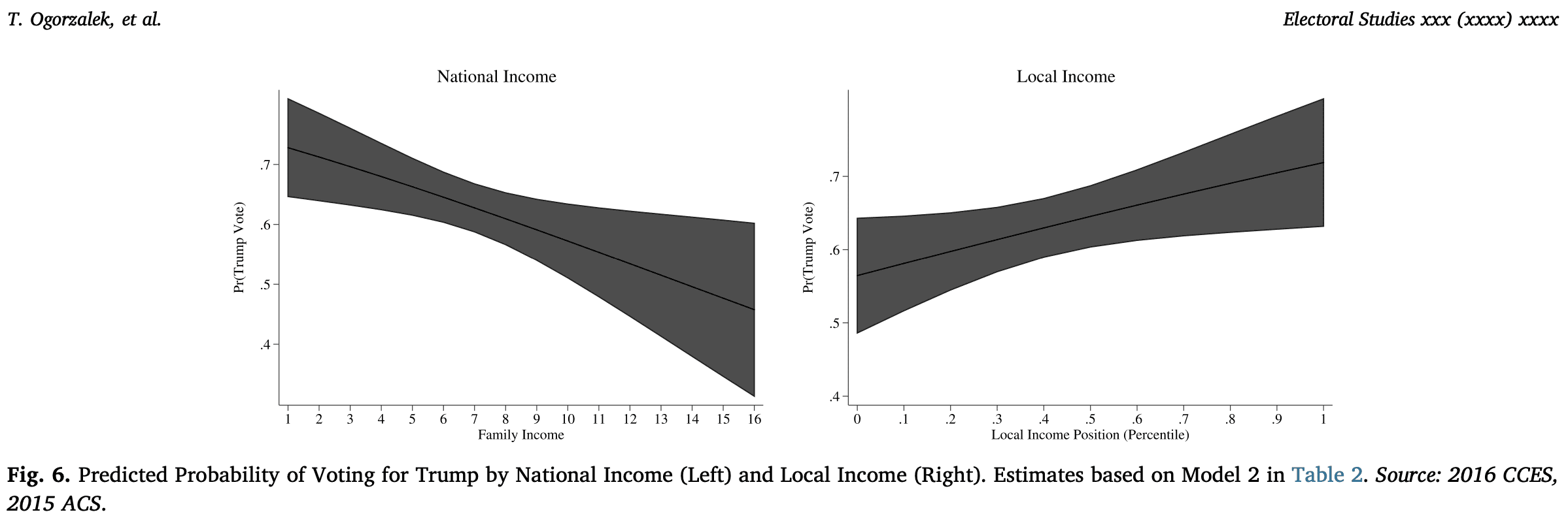
Nationally poor, locally rich: Income and local context in the 2016 presidential election

Thomas Ogorzaleka, Spencer Piston, and Luisa Godinez Puig write:

When social scientists examine relationships between income and voting decisions, their measures implicitly compare people to others in the national economic distribution. Yet an absolute income level . . . does not have the same meaning in Clay County, Georgia, where the 2016 median income was $22,100, as it does in Old Greenwich, Connecticut, where the median income was $224,000. We address this limitation by incorporating a measure of one’s place in her ZIP code’s income distribution. We apply this approach to the question of the relationship between income and whites’ voting decisions in the 2016 presidential election, and test for generalizability in elections since 2000. The results show that Trump’s support was concentrated among nationally poor whites but also among locally affluent whites, complicating claims about the role of income in that election. This pattern suggests that social scientists would do well to conceive of income in relative terms: relative to one’s neighbors.

Good to see that people are continuing to work on this Red State Blue State stuff.

P.S. Regarding the graph above: They should’ve included the data too. It would’ve been easy to put in points for binned data just on top of the plots they already made. Clear benefit requring close to zero effort.

The behavioral economists’ researcher degree of freedom

A few years ago we talked about the two modes of pop-microeconomics:

1. People are rational and respond to incentives. Behavior that looks irrational is actually completely rational once you think like an economist.

2. People are irrational and they need economists, with their open minds, to show them how to be rational and efficient.

Argument 1 is associated with “why do they do that?” sorts of puzzles. Why do they charge so much for candy at the movie theater, why are airline ticket prices such a mess, why are people drug addicts, etc. The usual answer is that there’s some rational reason for what seems like silly or self-destructive behavior.

Argument 2 is associated with “we can do better” claims such as why we should fire 80% of public-school teachers or Moneyball-style stories about how some clever entrepreneur has made a zillion dollars by exploiting some inefficiency in the market.

The trick is knowing whether you’re gonna get 1 or 2 above. They’re complete opposites!

I thought of this when rereading this post from a few years ago, where we quoted Jason Collins, who wrote regarding the decades-long complacency of the academic psychology and economics establishment regarding the hot-hand fallacy fallacy:

We have a body of research that suggests that even slight cues in the environment can change our actions. Words associated with old people can slow us down. Images of money can make us selfish. And so on. Yet why haven’t these same researchers been asking why a basketball player would not be influenced by their earlier shots – surely a more salient part of the environment than the word “Florida”? The desire to show one bias allowed them to overlook another.

When writing the post with the above quote, I had been thinking specifically of issues with the hot hand.

Stepping back, I see this as part of the larger picture of researcher degrees of freedom in the fields of social psychology and behavioral economics.

You can apply the “two modes of thinking” idea to the hot hand:

Argument 1 goes like this: Believing in the hot hand sounds silly. But lots of successful players and coaches believe in it. Real money is at stake—this is not cheap talk! So it’s our duty to go beneath the surface and understand why, counterintuitively, belief in the hot hand makes sense, even though it might naively seem like a fallacy. Let’s prove that the pointy-headed professors outsmarted themselves and the blue-collar ordinary-Joe basketball coaches were right all along, following the anti-intellectual mode that was so successfully employed by the Alvin H. Baum Professor of Economics at the University of Chicago (for example, an unnamed academic says something stupid, only to be shot down by regular-guy “Chuck Esposito, a genial, quick-witted and thoroughly sports-fixated man who runs the race and sports book at Caesars Palace in Las Vegas.”)

Argument 2 goes the other way: Everybody thinks there’s a hot hand, but we, the savvy social economists and behavioral economists, know that because of evolution our brains make lots of shortcuts. Red Auerbach might think he’s an expert at basketball, but actually some Cornell professors have collected some data and have proved definitively that everything you thought about basketball was wrong.

Argument 1 is the “Econ 101” idea that when people have money on the line, they tend to make smart decisions, and we should be suspicious of academic theories that claim otherwise. Argument 2 is the “scientist as hero” idea that brilliant academics are making major discoveries every day, as reported to you by Ted, NPR, etc.

In the case of the hot hand, the psychology and economics establishment went with Argument 2. I don’t see any prior reason why they’d pick 1 or 2. In this case I think they just made an honest mistake: a team of researchers did a reasonable-seeming analysis and everyone went from there. Following the evidence—that’s a good idea! Indeed, for decades I believed that the hot hand was a fallacy. I believed in it, I talked about it, I used it as an example in class . . . until Josh Miller came to my office and explained to me how so many people, including me, had gotten it wrong.

So my point here is not to criticize economists and psychologists for getting this wrong. The hot hand is subtle, and it’s easy to get this one wrong. What interests me is how they chose—even if the choice was not made consciously—to follow Argument 2 rather than Argument 1 here. You could say the data led them to Argument 2, and that’s fine, but the same apparent strength of data could’ve led them to Argument 1. These are people who promote flat-out ridiculous models of the Argument 1 form such as the claim that “all deaths are to some extent suicides.” Sometimes they have a hard commitment to Argument 1. This time, though, they went with #2, and this time they were the foolish professors who got lost trying to model the real world.

I’m still working my way though the big picture here of trying to understand how Arguments 1 and 2 coexist, and how the psychologists and economists decide which one to go for in any particular example.

Interestingly enough, in the hot-hand example, after the behavioral economists saw their statistical argument overturned, they didn’t flip over to Argument 1 and extol the savvy of practical basketball coaches. Instead they pretty much tried to minimize their error and try to keep as much of Argument 2 as they could, for example arguing that, ok, maybe there is a hot hand but it’s much less than people think. They seem strongly committed to the idea that basketball players can’t be meaningfully influenced by previous shots, even while also being committed to the idea that words associated with old people can slow us down, images of money can make us selfish, and so on. I’m still chewing on this one.

What does it take, or should it take, for an empirical social science study to be convincing?

A frequent correspondent sends along a link to a recently published research article and writes:

I saw this paper on a social media site and it seems relevant given your post on the relative importance of social science research. At first, I thought it was an ingenious natural experiment, but the more I looked at it, the more questions I had. They sure put a lot of work into this, though, evidence of the subject’s importance.

I’m actually not sure how bad the work is, given that I haven’t spent much time with it. But the p values are a bit overdone (understatement there). And, for all the p-values they provide, I thought it was interesting that they never mention the R-squared from any of the models. I appreciate the lack of information the R-squared would provide, but I am always interested to know if it is 0.05 or 0.70. Not a mention. They do, however, find fairly large effects – a bit too large to be believable I think.

I didn’t have time to look into this one so I won’t actually link to the linked paper; instead I’ll give some general reactions.

There’s something about that sort of study that rubs me the wrong way and gives me skepticism, but, as my correspondent says, the topic is important so it makes sense to study it. My usual reaction to such studies is that I want to see the trail of breadcrumbs, starting from time series plots of local and aggregate data and leading to the conclusions. Just seeing the regression results isn’t enough for me, no matter how many robustness studies are attached to it. Again, this does not mean that the conclusions are wrong or even that there’s anything wrong with the researchers are doing; I just think that the intermediate steps are required to be able to make sense of this sort of analysis of limited historical data.

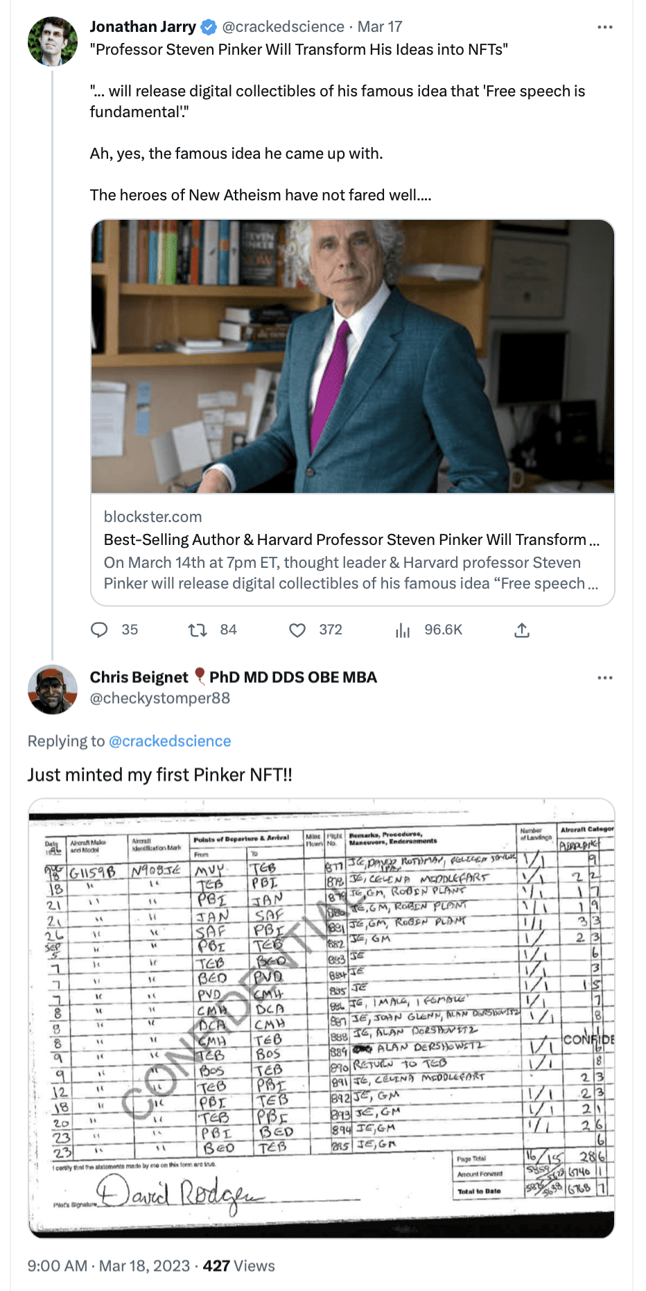
“On March 14th at 7pm ET, thought leader and Harvard professor Steven Pinker will release digital collectibles of his famous idea that ‘Free speech is fundamental.'”

A commenter points us to this juicy story:

John Glenn, huh? I had no idea. I guess it makes sense, though: after the whole astronaut thing ended, dude basically spend the last few decades of his life hanging out with rich people.

Following the link:

Two tiers will be available: the gold collectible, which is unique and grants the buyer the right to co-host the calls with Pinker, will be priced at $50,000; the standard collectibles, which are limited to 30 items and grant the buyers the right to access those video calls and ask questions to Pinker at the end, will be priced at 0.2 Ethereum (~$300).

Here’s the thing. Pinker’s selling collectibles of his idea, “Free speech is fundamental.” But we know from some very solid research that scientific citations are worth $100,000 each.

So does that mean that Pinker’s famous idea that “Free speech is fundamental” is only worth, at best, 0.5 citations? That doesn’t seem fair at all. Pinker’s being seriously ripped off here.

On the other hand, he could also sell collectibles for some of his other ideas, such as, “Did the crime rate go down in the 1990s because two decades earlier poor women aborted children who would have been prone to violence?”, “Are suicide terrorists well-educated, mentally healthy and morally driven?”, “Do African-American men have higher levels of testosterone, on average, than white men?”, or, my personal favorite, “Do parents have any effect on the character or intelligence of their children?” 50 thousand here, 50 thousand there, pretty soon you’re talking about real money.

All joking aside, I don’t see anything wrong with Pinker doing this. The NFT is a silly gimmick, sure, but what he’s really doing is coming up with a clever way to raise money for his research projects. If I had a way to get $50,000 donations, I’d do it too. It’s hard to believe that anyone buying the “NFT” is thinking that they’re getting their hands on a valuable, appreciating asset. It’s just a way for them to support Pinker’s professional work. One reason this topic interests me is that we’re always on the lookout for new sources of research funds. (We’ve talked about putting ads on the blog, but it seems like the amount of $ we’d end up getting for it would be not worth all the hassle involved in having ads.) As is often the case with humor, we laugh because we care.

And why is particular story this so funny? Maybe because it seems so time-bound, kind of as if someone were selling custom disco balls in the 1970s, or something like that. And he’s doing it with such a straight face (“* * * NOW LIVE . . . My first digital collectible . . .”)! If you’re gonna do it at all, you go all in, I guess.

P.S. Following the links on the above twitter feed led me to this website of McGill University’s Office for Science and Society, whose slogan is, “Separating Sense from Nonsense.” How cool is that?

What a great idea! I wonder how they fund it. They should have similar offices at Ohio State, Cornell, Harvard (also here), the University of California, Columbia, etc etc etc.

“Behavioural science is unlikely to change the world without a heterogeneity revolution”

Christopher Bryan, Beth Tipton, and David Yeager write:

In the past decade, behavioural science has gained influence in policymaking but suffered a crisis of confidence in the replicability of its findings. Here, we describe a nascent heterogeneity revolution that we believe these twin historical trends have triggered. This revolution will be defined by the recognition that most treatment effects are heterogeneous, so the variation in effect estimates across studies that defines the replication crisis is to be expected as long as heterogeneous effects are studied without a systematic approach to sampling and moderation. When studied systematically, heterogeneity can be leveraged to build more complete theories of causal mechanism that could inform nuanced and dependable guidance to policymakers. We recommend investment in shared research infrastructure to make it feasible to study behavioural interventions in heterogeneous and generalizable samples, and suggest low-cost steps researchers can take immediately to avoid being misled by heterogeneity and begin to learn from it instead.

We posted on the preprint version of this article earlier. The idea is important enough that it’s good to have an excuse to post on it again.

P.S. This also reminds me of our causal quartets.

Significance testing, the replication crisis, and the market for lemons

In an article, “Accounting research and the significance test crisis,” David Johnstone writes:

There are now hundreds of published papers and statements, echoing what has been said behind closed doors for decades, namely that much if not most empirical research is unreliable, simply wrong or at worst fabricated. The problems are a mixture of flawed statistical logic . . . fishing for significant results and publications, selective reporting . . . and ultimately the ‘‘agency problem” that researchers charged by funding bodies . . . are motivated more by the personal need to publish and please other researchers. Expanding on that theme, the supply of empirical research in the “market for statistical significance” is described in terms of “market failure” and “the market for lemons”.

He elaborates:

The problem for genuine research is that the process of learning while experimenting, gathering more data, improving proxies and experimental or statistical controls, and even things like cleaning data and removing outliers, can be explained equally by either “good” or “bad” science. To the outsider, they often look for all intents and purposes the same, which is a problem that will not go away in any research environment where work is published in elite journals even when it will not or cannot be replicated with new and independent data. The mechanics of information asymmetry, adverse selection and the market for lemons suggest that genuine research effort will go relatively unrewarded.

Here’s the background on that lemons thing:

A problem in the market for statistical significance is that the intrinsic qualities of the thing being sold are not observable to the buyer, much as in the Akerlof (1970) “market for lemons.” Many of the Akerlof corollaries apply. Information asymmetry between authors (sellers) and readers (buyers) will allow and reward opportunistic behaviours by authors and leave an adverse selection problem for journal editors in the case of papers rejected at other journals or sent to journals in more need of copy. Genuine researchers may be driven out of production, if they have no way to effectively “signal” the true quality of their work. In a limiting case, all papers published will be assumed to be “lemons”, as could hold true if enough genuine researchers find more rewarding applications for their skills and honesty, and the market will collapse.

Another finance analogy paints statistical researchers as akin to noise traders, where statistical noise masquerading as reliable evidence or a meaningful pattern can tempt belief and investment in a false lead. Even the investigator does not know when false assumptions (e.g. a false model) or pet hypotheses have been confirmed merely by luck or noise.

What’s amusing is that the “market for lemons” idea comes from economics, but empirical economics researchers are often entirely oblivious to these selection problems. Even famous, award-winning economists working on important problems can entirely miss the idea. Maybe the connection that Johnstone makes to the well-known lemons problem will help.

Reconciling evaluations of the Millennium Villages Project

Shira Mitchell, Jeff Sachs, Sonia Sachs, and I write:

The Millennium Villages Project was an integrated rural development program carried out for a decade in 10 clusters of villages in sub-Saharan Africa starting in 2005, and in a few other sites for shorter durations. An evaluation of the 10 main sites compared to retrospectively chosen control sites estimated positive effects on a range of economic, social, and health outcomes (Mitchell et al. 2018). More recently, an outside group performed a prospective controlled (but also nonrandomized) evaluation of one of the shorter-duration sites and reported smaller or null results (Masset et al. 2020). Although these two conclusions seem contradictory, the differences can be explained by the fact that Mitchell et al. studied 10 sites where the project was implemented for 10 years, and Masset et al. studied one site with a program lasting less than 5 years, as well as differences in inference and framing. Insights from both evaluations should be valuable in considering future development efforts of this sort. Both studies are consistent with a larger picture of positive average impacts (compared to untreated villages) across a broad range of outcomes, but with effects varying across sites or requiring an adequate duration for impacts to be manifested.

I like this paper because we put a real effort into understanding why two different attacks on the same problem reached such different conclusions. A challenge here was that one of the approaches being compared was our own! It’s hard to be objective about your own work, but we tried our best to step back and compare the approaches without taking sides.

Some background is here:

From 2015: Evaluating the Millennium Villages Project

From 2018: The Millennium Villages Project: a retrospective, observational, endline evaluation

Full credit to Shira for pushing all this through.

A bit of harmful advice from “Mostly Harmless Econometrics”

John Bullock sends along this from Joshua Angrist and Jorn-Steffen Pischke’s Mostly Harmless Econometrics—page 223, note 2:

They don’t seem to know about the idea of adjusting for the group-level mean of pre-treatment predictors (as in this 2006 paper with Joe Bafumi).

I like Angrist and Pischke’s book a lot so am happy to be able to help out by patching this little hole.

I’d also like to do some further analysis updating that paper with Bafumi using Bayesian analysis.

“Risk without reward: The myth of wage compensation for hazardous work.” Also some thoughts of how this literature ended up to be so bad.

Peter Dorman writes:

Still interested in Viscusi and his value of statistical life after all these years? I can finally release this paper, since the launch just took place.

The article in question is called “Risk without reward: The myth of wage compensation for hazardous work,” by Peter Dorman and Les Boden, and goes as follows:

A small but dedicated group of economists, legal theorists, and political thinkers has promoted the argument that little if any labor market regulation is required to ensure the proper level of protection for occupational safety and health (OSH), because workers are fully compensated by higher wages for the risks they face on the job and that markets alone are sufficient to ensure this outcome. In this paper, we argue that such a sanguine perspective is at odds with the history of OSH regulation and the most plausible theories of how labor markets and employment relations actually function. . . .

In the English-speaking world, OSH regulation dates to the Middle Ages. Modern policy frameworks, such as the Occupational Safety and Health Act in the United States, are based on the presumption of employer responsibility, which in turn rests on the recognition that employers generally hold a preponderance of power vis-à-vis their workforce such that public intervention serves a countervailing purpose. Arrayed against this presumption, however, has been the classical liberal view that worker and employer self-interest, embodied in mutually agreed employment contracts, is a sufficient basis for setting wages and working conditions and ought not be overridden by public action—a position we dub the “freedom of contract” view. This position broadly corresponds to the Lochner-era stance of the U.S. Supreme Court and today characterizes a group of economists, led by W. Kip Viscusi, associated with the value-of-statistical-life (VSL) literature. . . .

Following Viscusi, such researchers employ regression models in which a worker’s wage, typically its natural logarithm, is a function of the worker’s demographic characteristics (age, education, experience, marital status, gender) and the risk of occupational fatality they face. Using census or similar surveys for nonrisk variables and average fatal accident rates by industry and occupation for risk, these researchers estimate the effect of the risk variable on wages, which they interpret as the money workers are willing to accept in return for a unit increase in risk. This exercise provides the basis for VSL calculations, and it is also used to argue that OSH regulation is unnecessary since workers are already compensated for differences in risk.

This methodology is highly unreliable, however, for a number of reasons . . . Given these issues, it is striking that hazardous working conditions are the only job characteristic for which there is a literature claiming to find wage compensation. . . .

This can be seen as an update of Dorman’s classic 1996 book, “Markets and Mortality: Economics, Dangerous Work, and the Value of Human Life.” It must be incredibly frustrating for Dorman to have shot down that literature so many years ago but still see it keep popping up. Kinda like how I feel about that horrible Banzhaf index or the claim that the probability of a decisive vote is 10^-92 or whatever, or those terrible regression discontinuity analyses, or . . .

Dorman adds some context:

The one inside story that may interest you is that, when the paper went out for review, every economist who looked at it said we had it backwards: the wage compensation for risk is underestimated by Viscusi and his confreres, because of missing explanatory variables on worker productivity. We have only limited information on workers’ personal attributes, they argued, so some of the wage difference between safe and dangerous jobs that should be recognized as compensatory is instead slurped up by lumping together lower- and higher-tiered employment. According to this, if we had more variables at the individual level we would find that workers get even more implicit hazard pay. Given what a stretch it is a priori to suspect that hazard pay is widespread and large—enough to motivate employers to make jobs safe on their own initiative—it’s remarkable that this is said to be the main bias.

Of course, as we point out in the paper, and as I think I had already demonstrated way back in the 90s, missing variables on the employer and industry side impose the opposite bias: wage differences are being assigned to risk that would otherwise be attributed to things like capital-labor ratios, concentration ratios (monopoly), etc. In the intervening years the evidence for these employer-level effects has only grown stronger, a major reason why antitrust is a hot topic for Biden after decades in the shadows.

Anyway, if you have time I’d be interested in your reactions. Can the value-of-statistical-life literature really be as shoddy as I think it is?

I don’t know enough about the literature to even try to answer that last question!

When I bring up the value of statistical life in class, I’ll point out that the most dangerous jobs pay very low, and high-paying jobs are usually very safe. Any regression of salary vs. risk will start with a strong negative coefficient, and the first job of any analysis will be to bring that coefficient positive. At that point, you have to decide what else to include in the model to get a coefficient that you want. Hard for me to see this working out.

This has a “workflow” or comparison-of-models angle, as the results can best be understood within a web of possible models that could be fit to the data, rather than focusing on a single fitted model, as is conventionally done in economics or statistics.

As to why the literature ended up so bad: it seems to be a perfect storm of economic/political motivations along with some standard misunderstandings about causal inference in econometrics.

Contradictions within economic theory. All well known but still important and, I think, not taken as seriously as they should be.

Asher Meir writes:

Economists (like me) love models with “rational expectations”. In these models, all agents have mutually consistent expectations of some future economic equilibrium. If everyone expects that the outcome (which can be stochastic) is X, then it will be optimal for everyone to engage in choices that will result in X.

There can be no doubt that there is a certain logic in an equilibrium like this. So we spend a lot of effort and computer time to solve them. Because we don’t know what these equilibria look like.

Uh, wait.

If we don’t know what the equilibrium looks like, how is it possible that every single agent in the economy does know what it looks like?

I was the programmer for a model like this in the 1980s. This paradox bothered me a lot. Perhaps there is some satisfactory resolution to the paradox, but what drove me crazy even more was that no one was bothered by this obvious paradox. Alan Auerbach and Larry Kotlikoff were very happy to have me as a programmer because I was good at making it converge. Often you can’t prove that these models converge, but usually they are pretty well behaved and a decent programmer can nudge them towards an equilibrium. Then lo and behold, Larry and Alan and I would discover the equilibrium growth path is that had already previously been known to every single agent in the US economy and which underlied the US economy. . .

In the 1980s the models were pretty simple but today they are amazingly complicated. The stochastic ones are gridded and get you into the curse of dimensionality. Researchers expend a lot of effort trying to show that the model has a stable equilibrium, hopefully only one. But nobody seems to notice that while the researcher can impose a transversality condition on the model, s/he can’t impose one on the world.

As far as I can recall the only economist who was interested in this gaping black hole in our profession was Herb Simon. And nobody talked to Herb Simon.

My reply: Yes, I’ve heard this general argument made before. On one hand, individuals are modeled as Bayesian optimizers. On the other hand, actual Bayesian optimization is really difficult and requires Ph.D. statisticians etc. I had the impression that the usual resolution of this problem is to say that economic incentives push people toward optimality. Even though people do not individually behave optimally, any instances of non-optimality will be caught out by the market. This is the “as if” argument, no?

Meir:

No, that is not the problem I am pointing out.

The “as if” argument works not badly if our only problem is to optimize given known constraints. Human beings can’t maximize anything, all they have is crude climbing algorithms (as Herb Simon kept on trying to remind us), but they have a bunch of pretty good climbing algorithms and these could give a good approximation to maximization if that was what these algorithms were meant to emulate. (Fortunately for the survival of the human race, the algorithms are not actually meant to maximize our utility but rather our progeny.)

I am not at all denying that the problem you mention is grave and that practitioners extend the methodology beyond the places where it works “not badly” to places where it works badly. But the problem I am discussing is much worse.

In most economic models, the constraints depend on future outcomes, and those future outcomes depend among other things on the current expectations of millions of people. Once upon a time economists liked to actually ask people what those expectations were. That approach worked surprisingly well actually.

But then we had a rational expectations revolution and we adopted a new approach which has iterative models. These algorithms ask the following question: what current expectations are consistent with the current+future behavior which is optimal given the common knowledge of those expectations? This implies also that the expectations are shared. My expectations include my evaluation of what other people’s expectations are, and all these have to be self-consistent.

It is generally an incredible numerical headache to find those. When we do find a “rational expectations equilibrium”, we proceed to assume that those actually have been people’s expectations all along. We basically assume that RIGHT NOW each of millions of people know exactly what each of millions of people expects the future to be like. But we economists don’t know. But if we are extremely clever and solve an extremely intractable numeric iteration, we will know what people think RIGHT NOW.

So there are quite a few issues:

1. Economists like to assume that people are endeavoring to maximize something, but as far as I know there is little evidence that they do or should act that way. People have a variety of sophisticated algorithms which do lots of cool things but they don’t approximate maximizing any one-dimensional function. This assumption is not terrible if we are limiting ourselves to one narrow area of human endeavor. People do choose jobs to maximize their economic well-being and choose houses to maximize some intuitive basket of housing characteristics.

2. Then we assume that people actually find the maximum. Again, this is not a terrrible assumption as long as we don’t assume some kind of ridiculous precision. Though often we do, as your email points out.

3. The assumption that people have “rational expectations” in the sense of expectations that are common knowledge and self-consistent and are close to what some small-dimensional iterative numerical model with highly artificial assumptions will solve for does not seem to me to be remotely defensible. Maybe I am wrong.

I don’t want to spoil your fun, but I am guessing that lots of what you want to say was already said by Herb Simon and they even gave him a Nobel Prize for it but nobody paid attention and anyone who did I guess forgot. Do read some of his stuff.

While I’m in the business of selling gaping holes, here is another one, To the best of my recollection this doesn’t date to Herb Simon but rather back to the early 19th century and the early criticisms of utilitarianism. The following are the two most important insights Jeremy Bentham was selling:

1. A person’s well-being can be reduced to a one-dimensional number which is a function of his/her experiences. “Pushpin is as good as poetry”. Human psychology is basically the understanding that each individual is endeavoring to maximize his/her sensory pleasure.

2. Ethical conduct, to which all human beings should strive, is to maximize the sum total of humanity’s utility.

Wait, Jeremy, do people get utility from their utility or from everyone else’s utility? If the first, then how exactly do you expect them to strive to maximize the second? If the second, then perhaps people are going to spend little time playing pushpin and lots of time trying to bring about prison reform (a favorite of Bentham’s).

Once other people’s utility becomes part of my utility the whole thing blows up. Hopeless to expect you can converge. Consider the following sentiment which is common and perhaps universal: A person sees that his/her significant other is not really investing effort in making him/her self attractive: Feeling inside: “I want you to want me to want you”. This is an everyday sentiment which we all acknowledge and probably almost all of us experience. Try to put it into an equation to maximize! Our consumption is an argument to our utility function, OK. Other people’s consumption is an argument, nu. Now make other people’s UTILITY FUNCTIONS an argument. Sound easy? Now make the dependency of B’s utility function on A’s utility functions an argument in A’s utility function.

Meir continues:

A lot of these critiques have been around for a long time. Some for hundreds of years.

A lot of them turn on the normative/positive tension. Going back and forth between what we claim people do and what we think people should do and what we think is good for them.

If human conduct is not maximizing, then people aren’t making mistakes in the maximization and so utility maximization can’t really be an adequate normative framework. If as Herb Simon points out it is literally impossible that people should be “maximizers” since we are just computers with algorithms, then it is impossible that utility maximization can be an adequate normative paradigm.

Another problem is identifying utilitarianism with libertarianism. There is no particular reason to assume that freedom maximizes people’s utility. If North Koreans weren’t exposed to broadcasts from South Korea they would probably be a lot happier. Their belief that they are living in a heroic paradise led by a demi-god would be unchallenged. But libertarians are the first to favor giving people full information.

Lots to chew on here. I have more to say but I’m not quite sure what, so here’s everyone’s chance to discuss this in comments.

Sometimes it’s hard to talk about economists about this sort of thing because they get all defensive about it.

Yale prof thinks that murdering oldsters is a “complex, nuanced issue”

OK, this news story is just bizarre:

A Yale Professor Suggested Mass Suicide for Old People in Japan. What Did He Mean?

In interviews and public appearances, Yusuke Narita, an assistant professor of economics at Yale, has taken on the question of how to deal with the burdens of Japan’s rapidly aging society.

“I feel like the only solution is pretty clear,” he said during one online news program in late 2021. “In the end, isn’t it mass suicide and mass ‘seppuku’ of the elderly?” Seppuku is an act of ritual disembowelment that was a code among dishonored samurai in the 19th century.

Ummmm, whaaaa?

The news article continues:

Dr. Narita, 37, said that his statements had been “taken out of context” . . . The phrases “mass suicide” and “mass seppuku,” he wrote, were “an abstract metaphor.”

“I should have been more careful about their potential negative connotations,” he added. “After some self-reflection, I stopped using the words last year.”

Huh? “Potential” negative connotations? This is just getting weirder and weirder.

And this:

His Twitter bio: “The things you’re told you’re not allowed to say are usually true.”

On this plus side, this is good news for anyone concerned about social and economic inequality in this country. The children of the elites get sent to Yale, they’re taught this sort of up-is-down, counterintuitive stick-it-to-the-man crap, and to the extent they believe it, it makes them a bit less effective in life, when they enter the real world a few years later. Or maybe they don’t believe this provocative crap, but at least they’ve still wasted a semester that they could’ve spent learning economics or whatever. Either way it’s a win for equality. Bring those Ivy League kids down to the level of the rabble on 4chan!

And then this bit, which is like a parody of a NYT article trying to be balanced:

Shocking or not, some lawmakers say Dr. Narita’s ideas are opening the door to much-needed political conversations about pension reform and changes to social welfare.

In all seriousness, I’m sure that Yale has some left-wing professors who are saying things that are just as extreme . . . hmmmm, let’s try googling *yale professor kill the cops* . . . bingo! From 2021:

A Psychiatrist Invited to Yale Spoke of Fantasies of Shooting White People

A psychiatrist said in a lecture at Yale University’s School of Medicine that she had fantasies of shooting white people, prompting the university to later restrict online access to her expletive-filled talk, which it said was “antithetical to the values of the school.”

The talk, titled “The Psychopathic Problem of the White Mind,” had been presented by the School of Medicine’s Child Study Center as part of Grand Rounds, a weekly forum for faculty and staff members and others affiliated with Yale to learn about various aspects of mental health. . . .

“This is the cost of talking to white people at all — the cost of your own life, as they suck you dry,” Dr. Khilanani said in the lecture . . . “I had fantasies of unloading a revolver into the head of any white person that got in my way, burying their body and wiping my bloody hands as I walked away relatively guiltless with a bounce in my step, like I did the world a favor,” she said, adding an expletive. . . .

Dr. Khilanani, a forensic psychiatrist and psychoanalyst, said in an email on Saturday that her words had been taken out of context to “control the narrative.” She said her lecture had “used provocation as a tool for real engagement.” . . .

Don’t you hate it when you make a racist speech and then people take it out of context? So annoying!

The situations aren’t exactly parallel, as she was a visitor, not a full-time faculty member. Let’s just say that Yale is a place where you’ll occasionally hear some things with “potentially negative connotations.”

Getting back to the recent story:

Some surveys in Japan have indicated that a majority of the public supports legalizing voluntary euthanasia. But Mr. Narita’s reference to a mandatory practice spooks ethicists.

Jeez, what is it with the deadpan tone of this news article? “A mandatory practice” . . . that means someone’s coming to kill grandma. You don’t have to be an “ethicist” to be spooked by that one!

And then this:

In his emailed responses, Dr. Narita said that “euthanasia (either voluntary or involuntary) is a complex, nuanced issue.”

“I am not advocating its introduction,” he added. “I predict it to be more broadly discussed.”

What the hell??? Voluntary euthanasia, sure, I agree it’s complicated, and much depends on how it would be implemented. But “involuntary euthanasia,” that’s . . . that’s murder! Doesn’t seem so complex to me! Then again, my mom is 95 so maybe I’m biased here. Unlike this Yale professor, I don’t think that the question of whether she should be murdered is a complex, nuanced issue at all!

On the other hand, my mom’s not Japanese so I guess this Narita dude isn’t coming after her—yet! Maybe I should be more worried about that psychiatrist who has a fantasy of unloading a revolver into her head. That whole “revolver” thing is particularly creepy: she’s not just thinking about shooting people, she has a particular gun in mind.

In all seriousness, political polarization is horrible, and I think it would be a better world if these sorts of people could at least feel the need to keep quiet about their violent fantasies.

But, hey, he has “signature eyeglasses with one round and one square lens.” How adorable is that, huh? He may think that killing your grandparents is “a complex, nuanced issue,” but he’s a countercultural provocateur! Touches all bases, this guy.

Saving the best for last

Near the end of the article, we get this:

At Yale, Dr. Narita sticks to courses on probability, statistics, econometrics and education and labor economics.

Probability and statistics, huh? I guess it’s hard to find a statistics teacher who doesn’t think there should be broad discussions about murdering old people.

Dude also has a paper with the charming title, “Curse of Democracy: Evidence from the 21st Century.”

Democracy really sucks, huh? You want to get rid of all the olds, but they have this annoying habit of voting all time. Seriously, that paper reads like a parody of ridiculous instrumental-variables analyses. I guess if this Yale thing doesn’t work out, he can get a job at the University of California’s John Yoo Institute for Econometrics and Democracy Studies. This work is as bad as the papers that claimed that corporate sustainability reliably predicted stock returns and that unionization reduced stock price crash risk. The only difference is that those were left-wing claims and the new paper is making a right-wing claim. Statistics is good that way—you can use it to support causal claim you want to make, just use some fancy identification strategy and run with it.

A wistful dream

Wouldn’t it be cool if they could set up a single university for all the haters? The dude who’s ok with crush children’s testicles, the guy who welcomes a broad discussion of involuntary euthanasia, the lady who shares her fantasies of unloading her revolver . . . the could all get together and write learned treatises on the failure of democracy. Maybe throw in some election deniers and covid deniers too, just to keep things interesting.

It’s interesting how the university affiliation gives this guy instant credibility. If he was just some crank with an econ PhD and a Youtube channel who wanted to talk about killing oldsters and the curse of democracy, then who would care, right? But stick him at Yale or Stanford or whatever, and you get the serious treatment. Dude’s econometrics class must be a laff riot: “The supply curve intersects 0 at T = 75 . . .”

Controversy over an article on syringe exchange programs and harm reduction: As usual, I’d like to see more graphs of the data.

Matt Notowidigdo writes:

I saw this Twitter thread yesterday about a paper recently accepted for publication. I thought you’d find it interesting (and maybe a bit amusing).

It’s obvious to the economists in the thread that it’s a DD [difference-in-differences analysis], and I think they are clearly right (though for full disclosure, I’m also an economist). The biostats author of the thread makes some other points that seem more sensible, but he seems very stubborn about insisting that it’s not a DD and that even if it is a DD, then “the literature” has shown that these models perform poorly when used on simulated data.

The paper itself is obviously very controversial and provocative, and I’m sure you can find plenty of fault in the way the Economist writes up the paper’s findings. I think the paper itself strikes a pretty cautious tone throughout, but that’s just my own judgement.

I took a look at the research article, the news article, and the online discussion, and here’s my reply:

As usual I’d like to see graphs of the raw data. I guess the idea is that these deaths went up on average everywhere, but on average more in comparable counties that had the programs? I’d like to see some time-series plots and scatterplots, also whassup with that bizarre distorted map in Figure A2? Also something weird about Figure A6. I can’t imagine there are enough counties with, say, between 950,000 and 1,000,000 people to get that level of accuracy as indicated by the intervals. Regarding the causal inference: yes, based on what they say it seems like some version of difference in differences, but I would need to see the trail of breadcrumbs from data to estimates. Again, the estimates look suspiciously clean. I’m not saying the researchers cheated, they’re just following standard practice and leaving out a lot of details. From the causal identification perspective, it’s the usual question of how comparable are the treated and control groups of counties: if they did the intervention in places that were anticipating problems, etc. This is the usual concern with observational comparisons (diff-in-diff or otherwise), which was alluded to by the critic on twitter. And, as always, it’s hard to interpret standard errors from models with all these moving parts. I agree that the paper is cautiously written. I’d just like to see more of the thread from data to conclusions, but again I recognize that this is not how things are usually done in the social sciences, so to put in this request is not an attempt to single out this particular author.

It can be difficult to blog on examples such as this where the evidence isn’t clear. It’s easy to shoot down papers that make obviously ridiculous claims, but this isn’t such a case. The claims are controversial but not necessarily implausible (at least, not to me, but I’m a complete outsider.). This paper is an example of a hard problem with messy data and a challenge of causal inference from non-experimental data. Unfortunately the standard way of writing these things in econ and other social sciences is to make bold claims, which then encourages exaggerated headlines. Here’s an example. Click to the Economist article and the headline is the measured statement, “America’s syringe exchanges might be killing drug users. But harm-reduction researchers dispute this.” But the Economist article’s twitter link says, “America’s syringe exchanges kill drug users. But harm-reduction researchers are unwilling to admit it.” I guess the Economist’s headline writer is more careful than their twitter-feed writer!

The twitter discussion has some actual content (Gilmour has some graphs with simulated data and Packham has some specific responses to questions) but then the various cheerleaders start to pop in, and the result is just horrible, some mix on both sides of attacking, mobbing, political posturing, and white-knighting. Not pretty.

In its subject matter, the story reminded me of this episode from a few years ago, involving an econ paper claiming a negative effect of a public-health intervention. To their credit, the authors of that earlier paper gave something closer to graphs of raw data—enough so that I could see big problems with their analysis, which led me to general skepticism about their claims. Amusingly enough, one of the authors of the paper responded on twitter to one of my comments, but I did not find the author’s response convincing. Again, it’s a problem with twitter that even if at some point there is a response to criticism the response tends to be short. I think blog comments are a better venue for discussion; for example I responded here to their comment.

Anyway, there’s this weird dynamic where that earlier paper displayed enough data for us to see big problems with its analysis, whereas the new paper does not display enough for us to tell much at all. Again, this does not mean the new paper’s claims are wrong, it just means it’s difficult for me to judge.

This all reminds me of the idea, based on division of labor (hey, you’re an economist! you should like this idea!), that the research team that gathers the data can be different from the team that does the analysis. Less pressure then to come up with strong claims, and then data would be available for more people to look at. So less of this “trust me” attitude, both from critics and researchers.