Guess who’s getting the big-money donations in the Maine U.S. Senate race?

Just in time for July 4th, Tom Ferguson, Paul Jorgensen, Matthias Lalisse, and Jie Chen share the above graph and write:

What can one Senate race reveal about the hidden machinery of American politics? In Maine, donor patterns expose how campaign finance can shape party competition, political narratives, and the choices voters are asked to make long before ballots are counted. . . .

Platner is strongly supported by Senator Bernie Sanders and other progressives, while many establishment Democrats dislike him. Major media keep printing articles questioning his character. By contrast, Collins’ somewhat contradictory legislative history attracts less coverage. . . .

Our tabulations of the race show that Collins is much closer to a typical Republican pattern (or, to be fair, those of the Old Guard Democratic leaders [Nancy Pelosi and Chuck Schumer, along with Paul Ryan and Mitch McConnell]) in a key respect: the size profile of her donors. . . .

The Republican Senator from Maine is hugely dependent on very large donors. By contrast, Platner strikingly resembles Sanders: he attracts essentially no big money. Recently the numbers of billionaires supporting the candidates has emerged as an issue. A very few have supported Platner with small sums. Almost a hundred (counting spouses) have made contributions of varying sizes to Collins. The overall configuration is as shown [above] and is perfectly obvious.

They also report:

If you put aside contributions that are below the $200 threshold for disclosure, the percentage of money received from Maine donors differs sharply between the candidates. Senate elections have been nationalized for a long time. Contributions from Maine itself make up approximately 20% of all money for Platner; by contrast, Collins’ rate is slightly under 3%. (Not a misprint.) Her biggest contributors include a Who’s Who of prominent financiers in private equity and hedge funds, including Steve Schwarzman of BlackRock, Ken Griffin of Citadel, along with other well known Republican donors, including Larry Ellison of Oracle.

And they give an example of how this works:

A day after a Super Pac backing her received a $2 million dollar contribution from a private equity magnate who, according to press reports, stood to gain munificently from President Trump’s One Big Beautiful Bill, [Collins] provided a crucial vote to spring the bill out of committee. Then she loudly voted against it on the floor.

Another way of looking at this is to ask, why a person living outside of Maine give $100,000+ to Susan Collins? Roughly speaking, the following conditions are needed:
1. The donor has to be rich enough to be able to spare $100,000 as loose change.
2. It has to be legally possible to give this amount of money, or the perceived consequences of violating the law have to be minimal.
3. The donor has to consider Republican Party control of the U.S. Senate has to be important enough to be worth spending $100,000 to make a small change in the probability of this happening.
4. It has to be easy to write the check; that is, the donor does not need to get the agreement of many other people to release the money.
5. Any negative political, social, and economic consequences of revealing oneself to be a strong partisan have to be mild, compared to the perceived benefits of making the donation.

And in recent years these five conditions have increasingly been present:
1. There are more and more super-rich people who can spend $100,000 without blinking an eye.
2. The Supreme Court keeps liberalizing campaign finance laws, also the government has become much more encouraging and tolerant of corruption. On the rare occasions where people are prosecuted, they get off, and even on the rare occasions are imprisoned for corruption, they get pardoned.
3. With political polarization, the two parties are further apart than ever, and party-line voting in Congress has become the norm.
4. The money is being given by individuals, or by companies controlled by single individuals. It’s not like the old days, where, if General Motors made a campaign contribution, they’d need the coordination of some board of directors.
5. This last one is the most interesting. A flip side of partisan polarization is that, if you give a lot of money to the Republicans, it will piss off a lot of Democrats, and vice versa. Political independents might not be so happy either. One way out is that it’s becoming easier and easier to skirt the regulations and campaign in secret. Beyond this, I guess these donors have decided that the Republican business sphere is large enough that they can afford to alienate Democrats and independents. And Black Rock, Citadel, and Oracle are not primarily customer-facing businesses.

“Howard Lutnick gives top Cantor Fitzgerald jobs to his sons Brandon and Kyle” is a very clean example of meritocracy.

In a post about possible corruption in the government and finance sector, Paul Campos points to a news article entitled, “Howard Lutnick gives top Cantor Fitzgerald jobs to his sons Brandon and Kyle,” that features an adorable photo of the three Lutnicks standing next to a fashion model.

Campos labels this as, “The Meritocracy!”, and clearly he’s being ironic: his point is that it seems unlikely that these two twenty-somethings are really the people with the most merit needed to run this zillion-dollar company. All things are possible, but it would be an amazing coincidence if, among all the possible financial executives out there, that these two would happen to be the best.

And, sure, I get that.

But now I want to point to my old post on the topic, Meritocracy won’t happen: The problem’s with the “ocracy.”

The short version is that the news item, “Howard Lutnick gives top Cantor Fitzgerald jobs to his sons Brandon and Kyle,” is a very clean example of meritocracy. Lutnick Sr. had the merit (in whatever sense) that took him to the top of the heap, and he used that merit to get jobs for his kids: that’s the “ocracy” part.

If all that merit did was get you top jobs and lots of money, that’s not meritocracy, that’s just merit-based employment and pay. What makes it “meritocracy” that the people with the merit don’t just get nice jobs, they also get to be in charge of everything (”ocracy”). And one thing you do when you’re in charge is take care of your kids!

As Mark Palko discussed over ten years ago, our society seems to have become more tolerant of nepotism. Or maybe the point is that nepotism has always been a thing, but in recent years there’s been more of an effort by rich people and the news media to portray nepotistic hires as having special merit of their own. This is not to say that children of the successful cannot make great contributions themselves—John Quincy Adams comes to mind, also Julian Lennon had that cool song a few decades ago where he sounded just like his dad, so that’s something too. And then there was Oliver Wendell Holmes, Jr., who surpassed his famous father in achievements. And Alexander of Macedon didn’t do so bad either.

Anyway, “meritocracy” implies that the people with merit rule society, and they’ll use their power to help their kids.

Nepo babies aren’t a counterexample to meritocracy, they’re a central part of it.

The new rule in economics: One star is p < 0.20, two stars is a set of steak knives, three stars is you're fired.

Someone pointed me to a series of applied economics papers:

1. George Borjas and Nate Breznau, Ideological bias in the production of research findings:

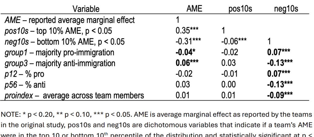
Our study exploits an opportunity to observe 158 researchers working independently in 71 teams during an experiment. After being asked their position on immigration policy, they used the same data to answer the same empirical question: Does immigration affect public support for social welfare programs? . . . teams composed of pro-immigration researchers estimated more positive impacts of immigration on public support for social programs, while anti-immigration teams estimated more negative impacts. The differences arise because different teams adopted different model specifications. . .

The results include an unusual labeling of statistical significance:

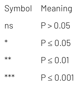
Usually it’s one star for p < 0.05, two stars for p < 0.01, as here:

or here:

These are not intended to be authoritative references; they just turned up in a quick search. The point is that 0.05 is the usual standard. Using 0.10 is a way of manufacturing a “statistically significant” result when you don’t have it in your data (as here). In the case of the Borjas and Breznau paper, the data were too variable to get a conventionally strong result, but they still wanted to get it published, and so they shifted the stars. I’m surprised that the reviewers didn’t catch it!

Don’t get me wrong. I don’t think people should be using statistical significance, at any level, as a threshold. To get a sense of my perspective you can read our paper, Abandon Statistical Significance. Even if you have an estimate that’s just one standard error from zero, that’s still evidence of the direction of the effect, as long as no selection is going on.

2. Katrin Auspurg and Josef Brüderl, Fragile Evidence for an Ideological Bias in the Production of Research Findings: Comment on Borjas and Breznau:

Although we were able to reproduce B&B’s numerical results, our reanalysis shows that the reported association is not robust. Specifically, the association hinges on a coding error. Data from four teams that contradict the ideology hypothesis were excluded from the analysis due to idiosyncratic variable coding. Correcting this error renders the ideology effect no longer statistically significant. Also, B&B employed a different outcome variable and weighƟng scheme to that used in a previous paper based on the same data. These two analytical decisions further contribute to the observed ideology effect. Correcting the coding error or using the same specification as in the previous paper renders the ideology effect indistinguishable from zero. . . .

They also go with the 10% significance level, I guess to be consistent with the original paper?

3. Nate Breznau and George Borjas, A Lack of Robustness in Robustness Checking from Auspurg and Brüderl:

In our published paper, we explicitlyacknowledged the limitations of our findings which are based on secondary data and a small sample. After examining Auspurg and Brüderl’s claims, we conclude that they have not presented any new evidence that warrants any correction to our conclusions. . . .

This rejoinder includes the table at the top of this post, in which the significance level has now crept up to 0.20.

I’m anticipating a few more rounds of this, culminating in a table by Breznau and Borjas in which anything with a two-sided p-value of less than 0.5 is given a star. Everybody’s a winner!

P.S. Just kidding in the title of the post. This “p < 0.20" thing isn't really the new rule in econ; it's just something from this one paper. It may be that its authors got some special exemption from the 0.05 threshold.

Gambling provides a gentle rocking of the emotions to put you in a pleasant baby-like state

A commenter recommended the book, Addiction by Design: Machine Gambling in Las Vegas, by the anthropologist Natasha Dow Schüll, and I checked it out of the library. It’s a study of people who play slot machines and video poker, focusing on the locals: Vegas residents who have some low-level gambling addictions as part of their lives.

Nowadays, I guess that much of this business has been supplanted by machine gambling that you can do on your phone in the comfort of your own home. But the market for gambling must be far from being tapped: I imagine that there are many millions of potential gambling addicts out there, available to be hooked by some form of gambling or another.

As a statistician, I have mixed feelings about gambling. Ever since I was a kid, I’ve thought that probability is cool, and I like to bet. When we were kids we had a toy roulette set that we would play (just betting chips, not real money) and I’ve enjoyed poker and informal sports betting. The last time I’ve bet on anything was about 20 years ago, but that’s just more me getting older than anything else.

At the same time, there are all these addicts, and all the people who might not be addicts but who still degrade their standard of living, not to mention reward evil people (even if they’re pleasant as invididuals, they’re in an evil business; sorry, Nate!). And it just keeps getting worse.

To a statistician, this is all an endlessly fascinating topic: the odds and all that, but also whatever it is in people’s brains that motivate them to spend thousands of dollars on lottery tickets, etc.

As Schüll writes in her book, the popularity of machine gambling (which she says is the source of the majority of casino gambling profits in Vegas) is particularly puzzling in that people are just pulling the lever over and over again, without the sense of human context or any feeling of agency.

There’s also the interaction between the players and the people who make money from the machines:

For extreme machine gamblers, the experience of play is an end in itself–an “autotelic” zone beyond value as such, in that “no other reward than continuing the experience is required to keep it going.” Conversely, for the gambling industry the zone is a means to an end; although it carries no value in and of itself, it is possible to derive value from it. . . . In effect, gamblers’ drive to remain indefinitely suspended in the zone is rerouted, via the technological detours of the gambling industry, toward a destination of complete depletion.

It’s not just “the technological detours of the gambling industry,” it’s also politics: the industry doing what it takes to keep all this going, a gradual effort over many decades that continues to this day.

Later, Schüll summarizes:

Gambling addicts play machines to suspend themselves in a state of equilibriated affect.

This seems pretty accurate.

I would just add two things.

First, this equilibrium is not flat. It’s periods of stress, punctuated with the occasional excitement of winning and the frequent relaxing calm of losing. The best analogy I can think of is the way that a baby is calmed, not by lying completely still, but by being rocked in a somewhat irregular fashion.

Second, stakes matter. That “state of equilibriated affect” can only be achieved when real money is involved. I guess this is related to the phenomenon of habituation in drug exposure. Schüll talks with someone who started on a zero-stakes poker video game but them moved to the machines that take real dollars. We discussed this general idea recently in our post, Why isn’t it possible to play a fun and serious game of poker not for money?

It’s a good thing that babies don’t work that way–you can rock them a reasonable amount and they’ll be happy. No need to keep upping the stakes until the crib does a loop and the baby flies out the window. Although I guess that might happen if there were money in it.

The New York Knicks and the martingale property of calibrated probability forecasts (with some simulation and R code)

This long post covers four topics:

1. The Knicks’ stunning series of come-from-behind victories to win the NBA title in 5 games;

2. The martingale property of probability forecasts;

3. An example of learning from simulation;

4. How we (sometimes) do research in probability and statistics.

I don’t know enough about this blog’s audience to know which of the four topics will appeal to most of you. For the internet as a whole, it’s #1; for most of you, it might be #3.

I’m interested in all four, which is why I’m writing this all up right now. I’m embarrassed to say that it took several hours to do this. I was originally planning to post this Sunday morning after the game but it took time for me to get to the task. Most of the effort came from writing the code, not from writing the text. And there’s actually not much code, as you can see if you scroll to the end of this post. The main effort was not figuring out the syntax or even debugging (although there was some of that) but in working out what I wanted to be coding in the first place.

On the plus side, this is research I’ve been wanting to do for awhile, so (a) I don’t think this effort is wasted, even beyond whatever educational and entertainment value if has for you, and (b) I learned a bit from this already. Looking at data is always good; experimenting with simulation is always good.

Ok, here goes.

The NBA finals

Hey, remember this, from game 4 of the recent NBA finals:

Or the trajectory of the game that came after:

Just for completeness, here are the traces for games 3, 2, and 1, also courtesy of ESPN:
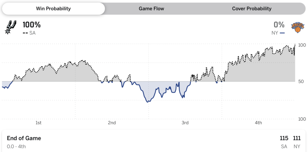
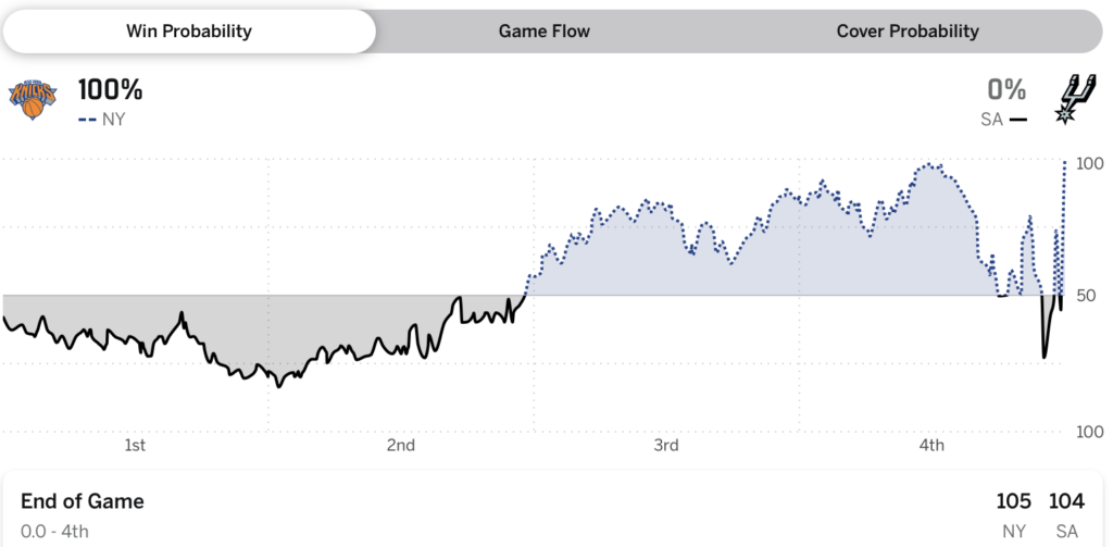
In game 4, the Spurs at one point were estimated to have a 99.6% chance of winning. But, as you might have heard, they lost.

Extreme win probabilities

Were those stated win probabilities too extreme?

On one hand, sure, unusual events happen on occasion. If you have a 0.4% chance of losing, that’s something that should happen 1 in 250 times, and there were a lot more than 250 basketball games just in this past season. On the other hand, very unusual event are supposed to happen only very rarely, and there was a point in the third quarter of game 4 where ESPN’s algorithm gave the Spurs a 97.1% chance of winning, a point in game 1 where the Spurs were given a 94.1% chance. There was a moment in game 2 where the Knicks were assigned a 98.2% chance of winning, and, sure, they did win that one, but given that the final score was 105-104, after being tied 97-97 and 104-104, it seems in retrospect that this 98.2% was a bit overconfident.

Should we be suspicious of these probabilities? One way to ask this question is to check calibration: if we collect all game situations where a team has a 99.6% of winning, are they winning 99.6% of the time?

On the other hand, I’m picking the most extreme values of these win probabilities. You should get calibration of win probabilities at any time, and it’s ok to condition on them, but only to condition on what came before.

That is, if we look at win probabilities at the end of the first quarter, or at the end of the first half, or at the end of the third quarter, they should be calibrated. And if you look only at win probabilities only when they’re greater than 99%, they should be calibrated. And if you look only at win probabilities when they are the maximum for the game so far, they should be calibrated. But it’s not clear to me that you should expect calibration for win probabilities selected to be the maximum for the entire game, because if the win probability at time t is p(t), and you condition on the event p(t) < p(t_0) for t > t_0, that could provide information. It’s tricky.

The martingale property of probability forecasts

We wrote about this in section 1.6 of our 2020 article, Information, incentives, and goals in election forecasts:


And it also came up in some blog posts:

from 2020: Do we really believe the Democrats have an 88% chance of winning the presidential election?

from 2020: More on martingale property of probabilistic forecasts and some other issues with our election model

from 2024: “Unusual Betting Patterns With Several Temple Games”: It’s martingale time, baby!

also from 2024: It’s martingale time, baby! How to evaluate probabilistic forecasts before the event happens? Rajiv Sethi has an idea. (Hint: it involves time series.)

I’d expect ESPN’s win probabilities to be closer to calibrated than prediction-market odds or model-based election forecasts. Prediction markets depend on the bettors and there’s no reason to expect calibration, at least not until the market is fully mature in some way. Model-based election forecasts are based on approximate models that have known pathologies (for example here), so they won’t be universally calibrated. ESPN’s probabilities won’t be calibrated either–they too are based on an imperfect model–but I assume it’s model has been trained on tons of data so I don’t think it should be far off.

If someone could send me the moment-by-moment estimated win probabilities from some large database of basketball games, we could take a look.

In the meantime we can get some intuition by simulating from a mathematical model where we can compute win probabilities exactly.

Simulating the process

Assume a simple Brownian motion with drift, where the score differential y(t) starts at y(0) = 0 and then takes a continuous random walk so that y(t) ~ normal(delta*t, sigma*sqrt(t)). We’ll scale t to be in minutes, so the game goes from t=0 to t=48, with the winner being determined by y(48). The drift is then delta=point_spread/48, because this is the expected final score differential before the game has started. And we’ll set sigma=2, which seems reasonable: 2*sqrt(48)=13.8, so that the sd of the final score differential is approximately 14 points.

One cool thing about this model is that the win probability can be trivially computed given the score differential at any point in the game.

How wrong can you be?

To demonstrate, I’ll show the results–the score and the win probability during the game–for 18 independently simulated games. For simplicity I’ll assume the point spread is 0, so the two teams are always assumed to be evenly matched. And I’ll step through the game 10 times per minute, thus approximating the game as a sum of 480 independent increments.

The code is below; here are the results:
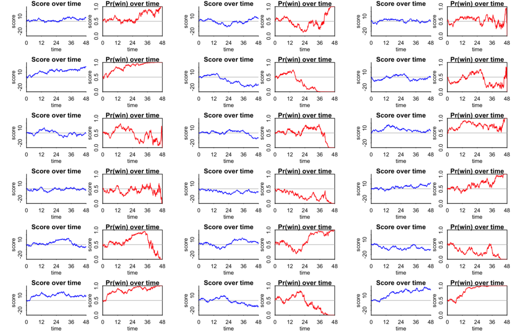
I don’t know enough about basketball to have a sense of how plausible these are as game outcomes (setting aside the lack of discreteness in the score; we used a continuous model so that we could more easily compute the relevant probabilities analytically). They don’t look too much like the Knicks-Spurs game except for that one simulation near the lower left of the plot, where the “Spurs” led by 10 points into the third quarter, maxing out with a win probability of 95.6% before eventually losing.

To get a broader picture, I simulated 10,000 games. (Just as a reference point, there are 30 NBA teams, so there are 82*30/2=1230 regular season games each year.)

For each game, I computed “max_p_wrong”: the highest win probability assigned to the game’s eventual loser. In my simulation, every game starts with a 50/50 probability–remember, for simplicity I’m always assuming a point spread of 0–so max_p_wrong must be somewhere between 0.5 and 1. Here’s what comes out:
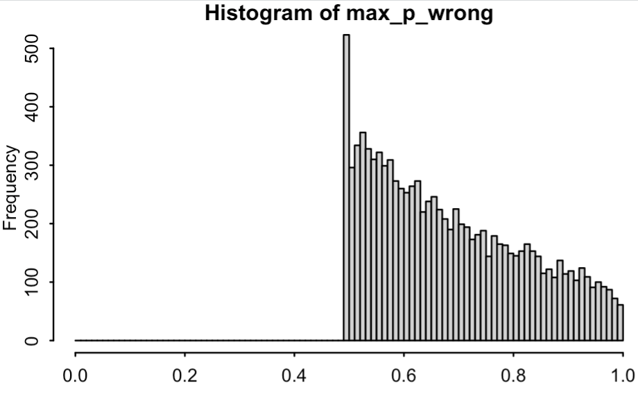
So, extreme wrong probabilities are not unheard of. How common are they? Out of these 10,000 games, 61 had max_p_wrong greater than 99%. That is, in 0.6% of games, the eventually-losing team exceeds the threshold of 99% win probability during some point in the game.

This result should go up if we move to continuous updating. But we’re already updating 10 times a minute. Increasing this schedule to 50 times a minute increases Pr(max_p_wrong > 0.99) to 0.0075, and increasing to 100 times a minute takes it to 0.0076, so my guess is that this is roughly the continuous limit.

OK, just to check, I’ll simulate 100,000 games, and now Pr(max_p_wrong > 0.99) is 0.0072 with 10 updates a minute, or 0.0084 with 50 updates per minute. So I’ll go out on a limb and say that if we were to compute the exact probability under continuous updating, we’d get 0.0085.

This was a surprise. Before doing this simulation, I was assuming that the probability of p_win exceeding 99% in for the eventual loser at any time in the game would be more than 1% because of selection. I guess my intuition was wrong. Maybe it has to do with the fact that I’m conditioning on which team wins. (Of course, if you go the other way, the probability of p_win exceeding 99% for the eventual winner is 100% in the continuous limit, because with epsilon of a second left in the game the winner will almost certainly be known.)

So, yeah, the above graph is kind of interesting. Under our model, most games won’t stray too far into retrospectively-embarrassing probability estimates, but it can happen sometimes.

It would be interesting to compare the above graph with what you’d get from a database of game-odds data from ESPN or whatever.

Just to be clear: there’s no reason to think that the above graph represents any sort of universal property of martingales. It’s a very specific model! But you have to start somewhere. Also, the existence of various central limit theorems makes me hold out the hope that this could be a general result under some appropriately restricted class of continuous martingale processes. It’s a research question!

A surprising uniform distribution

To get some further understanding of the process, I gathered the win probabilities after the end of each of the three quarters for the 10,000 simulated games. Below are histograms of these probabilities and calibration plots:

Unsurprisingly, the calibration is fine. After all, the probabilities are computed from the same model that the data are drawn from. Indeed, even the apparent anomaly in the lower-left plot is just a small-sample artifact which disappears when we up the number of simulations to 100,000.

More interesting are the histograms. It makes sense that, as the game goes on, the distribution of win probabilities starts at 0.5, then gradually bunches up at 0 and 1. Indeed, at the end of the fourth quarter the win probabilities are exactly 0 and 1.

But it’s funny how the distribution of win probabilities is exactly uniform at halftime. There must be a direct mathematical argument giving intuition for that result; it’s too perfect to just be an accident.

Lots more research to be done here:

– Generalizing beyond the continuous model to allow discrete scoring changes.

– Generalizing beyond the random walk; there’s no reason the model needs to be Markovian.

– Are there general statements that can be made about these distributions of win probabilities under arbitrary martingale processes? I’m guessing there are some results. At least, there should be some inequalities and limit theorems.

– Looking at real data from basketball, other sports, and other realms, including election forecasts and prediction markets.

Our ultimate aim here is to come up with a general measure of departure from the martingale property of probability forecasts. We want something that can be applied to any dataset, obviously with more precision as the series get longer, more finely-spaced in time, and when replications are available (as in those thousands of basketball games).

P.S. Here’s the R code to make the above simulations and graphs:
Continue reading

Ph.D. student opening in Sweden on Earth Observation, Data Science, and AI for poverty estimation

Adel Daoud writes:

I’m writing to ask for your help circulating a PhD opening in my group at Chalmers, the AI and Global Development Lab (www.aidevlab.org). The position is in Earth Observation, Data Science, and AI for poverty estimation, the Data Science and AI division (Department of Computer Science and Engineering). We are looking for candidates with a strong grounding in data science, computer science, deep learning, statistics, or similar— remote sensing experience and causal inference are welcome bonus.

Ad and application portal: https://www.chalmers.se/en/about-chalmers/work-with-us/vacancies/?rmpage=job&rmjob=14818&rmlang=UK
Deadline: 20 June 2026.

Here’s the description of their center:

The AI & Global Development Lab fuses AI with Earth Observation to illuminate the causes and consequences of human development across time and space.

Our interdisciplinary team, comprising data scientists, computer scientists, and social scientists, develops methods to better understand the multi-scale dynamics of pressing global issues, including poverty, conflict, sustainability, and the effectiveness of policy interventions.

By analyzing satellite imagery from 1984 to the present, AI search agent swarms for large-scale knowledge discovery, and other planetary-scale sources, we are reconstructing historical and geographical development trajectories at a level of detail never before possible, working to offer new insights into the changing face of development worldwide.

We also invite you to visit PlanetaryCausalInference.org for more information about the causal arm of our project.

They call it “Planetary causal inference,” which seems to fit the themes of this blog.

Capitalism: On its last legs or healthy enough to be milked?

In The Strange Death of Tory England, a book full of great lines, Geoffrey Wheatcroft writes,

Just as the labour movement had never been quite sure whether the capitalist system was on its last legs and needed only a final push to be toppled, or was healthy enough to be milked over and again, so the cultural-intellectual left had never quite decided whether it liked increasing prosperity or not.

I like the above quote, and I would add something analogous for conservatives, that they have never been quite sure whether the capitalist system is an amazing wealth machine with even low-income people being rich on an absolute scale, or whether the system is so fragile that people can barely afford to pay their taxes and that any particular tax or regulation will bankrupt the system. Unfortunately, try as I might, I can’t manage to phrase this as aphoristically as Wheatcroft did.

I suppose that every political movement must balance between triumphalism and alarmism. For another example, environmentalists will announce their progress in protecting the environment and warn of all the horrible things that will happen if more isn’t done. From the other direction, business groups will say that we can’t afford to protect the environment (we want jobs, not owls) but at the same time insist that the environment is better than ever.

The political science research project all this would be to study these ideologies more systematically and see which groups follow different patterns in their statements.

“Are prediction markets causing more harm than good?”

The other day I was invited to an “anti-debate” on the above topic, scheduled for this afternoon. I’d not heard about the concept of an anti-debate before; here’s the description:

The Anti-Debate is a new format for debate where participants build on each other’s insights, so that greater complexity can emerge.

Despite its name, the Anti-Debate is not anti-debate. It actually starts out like a traditional debate, with opening statements and rebuttals. But then it goes further — guiding participants to explore how they might integrate their perspectives into a bigger picture. Hence our tagline: First Debate, Then Elevate.

Sounds reasonable to me. They refer to the concept of steel-manning, and I’m skeptical of that, but I agree that standard debate formats have problems (just read The Topeka School!) and I’m very open to this sort of alternative.

The organizer, Winter Ku, referred to my posts on “the statistical skepticism about betting markets versus polls (self-reinforcing prices, thin volume), and more recently the integrity and harm concerns in your ‘Uh oh prediction markets’ writing, e.g. manipulation, the absence of insider-trading rules, and the gambling-like risks to vulnerable users,” and it seemed like it would be fun to have a chance to speak on this with several hundred people who might well be inclined to disagree with me. At the very least, I’d get some good questions, lots of pushback, and I’d probably change my mind about a few things.

The anti-debate was to be held at Manifest, an annual festival about prediction markets and forecasting at the same California location that had this blogging workshop a couple months ago. Unfortunately I was only invited to the Manifest thing a couple days ago and I wasn’t able to fly out on such short notice.

I hope the anti-debate goes well without me! Actually, it’ll probably go better without me than with me. I think I’m a careful and interesting writer with lots of good ideas, but I don’t know how well I’d do in a live debate. I imagine I’d get flustered. On the other hand, sharing objections to prediction markets, in front of a crowd coming from a much different perspective than me, but open to listening, could possibly do some good, as well as being a learning experience for me.

So maybe next year! I don’t know if they’ll put the anti-debate up on youtube or whatever; if so, it would be interesting to see the arguments on both sides.

P.S. I came across this entertaining and meandering report from Peter Miller describing this Manifest conference. So now I know what I missed!

Noem’s Razor and why I think the concept of “unintended consequences” is overrated

I was thinking more about Noem’s Razor (“Never attribute to stupidity that which is adequately explained by malice”) and it reminded me of that “Unintended consequences” often were actually intended, a principle that I discussed back in 2008 in the context of Freakonomics, that reliable purveyor of conventional wisdom; see also here and here.

One of my general problems with the concept of “unintended consequences” is that it so often seems to be used either as an argument against a proposed reform (recommending to not do this seemingly good thing because of its unintended consequences; what Albert Hirschman called the “perversity thesis” in his classic book, The Rhetoric of Reaction) or as a way to get evildoers off the hook by arguing that their bad actions were actually the unintended consequences of somebody’s good intentions.

I have a similar problem with Hanlon’s Razor (“Never attribute to malice that which is adequately explained by stupidity”). Often Hanlon’s Razor applies, that’s for sure, but I also think it can be a way to let people off the hook.

Also, often the simpler explanation is the right one. In the motivating example for Noem’s Razor, someone attributed the lethal behavior of the immigration police in Minneapolis as a “Sad case of poor incentive design (ICErs create expensive externalities bc of legal, reputation. etc costs of processing bad detentions and arrests. Textbook amateur mistake.”–but it seemed to me more likely that those police were doing what the government wanted. So the incentives (by which the agents can break the law without fear of consequences) worked directly. There’s no evidence that the consequences were unintended. The political consequences may well have been not as desired, but I see that as more of a political miscalculation than anything else.

As the economists say, when there’s a policy that seems like it doesn’t make sense, think more carefully about the incentives. And of course this policy applies much more generally, as in the literature on regulatory capture.

I don’t buy the argument that the nice guys are the real assholes. I think the assholes are usually the real assholes.

That doesn’t mean I think that all purported do-gooders are actually doing good–see here, for example. People need to be evaluated based on what they do, not what they say.

“Rationally Turbulent Expectations”

Kent Osband writes:

About 15 years ago you kindly linked an article I wrote on “rational turbulence.” I’d like to let you know that I have recently summarized much more research along these lines in a short book Rationally Turbulent Expectations.

I have published it as cheaply as color printing allows and also posted all chapters for free on ssrn, starting with this overview.

The main finding, summarized in the first few pages of Chapter 4, is that–once we allow for even tiny doubts about the the stability of an iid process–Bayesian learning has calm and turbulent phases, with fast learning more turbulent. It explains why differences in opinion between two reasonable people often widen before they narrow. I think this deserves broader attention in that people can learn to disagree more respectfully.

Hardly anyone will listen to me but many listen to you, so I am hopeful you will persuade yourself of this quickly and help persuade others.

I clicked through and took a look. Lots of things there resonate with various ideas I’ve discussed various times without ever fully thinking them through. For example:

“Words like ‘ahead’ and ‘forward’ that point to space in front of us also point to future time. However, that isn’t the only way to align directions”: This reminds me of the idea discussed here that there’s a logic of causality going forward in time and a logic of inference going backward in time. Generative models in statistics are a way of going from one of these to the other.

“Most surprises are outliers from a still intact trend. We tweak the next round of forecasts and move on. Occasionally the surprises get under our skin. They shock us less by their size than their persistence. They make us suspect that what we thought of as a rare outlier is now the new norm”: This reminds me of the ideas of Shewhart, Deming, etc., on quality control, an approach to statistics which I think is important and underrated.

“Contemporary finance theory rests on an unstable truce between two opposing schools. . . . The Rational Expectations school treats the market as a knowledge machine that assesses risks correctly and prices them appropriately. The Behavioral Finance school treats the market as a ship of fools prone to long stretches of complacency and short bouts of panic”: This reminds me of what I’ve called the two modes of reasoning in microeconomics: people are sometimes considered to be rational, so that the role of economists is to observe and analyze behavior and, from that, deduce values and motivations; and sometimes people are considered to be irrational, and the role of economists is to set them straight. Either way, the economist (or “freakonomist”) is portrayed as a culture hero, either in protecting us from pinheaded academics who don’t trust the ordinary Joe to make his own damn decisions, or in helping people avoid deadweight losses all around them.

Osband frames the economy in terms of turbulence, which fits in well with the idea that economics occurs on the phase transition of equilibrium. “Turbulence” seems like an appropriate term.

I don’t have the energy to read the whole book–I guess there’s an economic message there too!–so I can’t say more, but I’m happy to spread the word, and if you’re interested you can take a look into it yourself.

No, Bayes does not like Mayor Pete. (Pitfalls of using implied betting market odds to estimate electability.)

This one’s from 2019, but it’s worth reposting given recent interest in prediction markets.

The story starts with a post from economist Greg Mankiw, who wrote:

Who has the best chance of beating Donald Trump? A clue can be found using Bayes Theorem.

Here is the logic. Let A be the event that a candidate wins the general election, and B be the event that a candidate wins his or her party’s nomination. Predictit gives us the betting market’s view of P(A) and P(B). It is a safe assumption that P(B|A) = 1, that is, a candidate can win only if nominated. We can then use Bayes theorem to compute P(A|B), the probability that the candidate will win the general election conditional on being nominated.

So here are the results for P(A|B) as of now:

Buttigieg 0.80
Biden 0.77
O’Rourke 0.67
Sanders 0.65
Booker 0.60
Yang 0.60
Harris 0.57
Warren 0.44

That is, the betting markets suggest that Mayor Pete would be the strongest candidate if nominated, with Joe Biden close behind. (Of course, these numbers will bounce around as the prices in betting markets change.)

By the way, when I [Mankiw] did a similar calculation in 2006, Bayes liked Barack Obama.

I copied Mankiw’s post in its entirety, with the only change being that he wrote P(A / B) etc., and I changed the slash to the vertical bar, P(A|B). (Are there people who write conditioning using a slash rather than a vertical bar? I had no idea. P(A|B) is more standard, I believe. In the above post, Mankiw links to the wikipedia page which uses the P(A|B) notation. No big deal, it just seemed odd to me.)

Anyway, I think the above set of calculations is a great example for teaching conditional probability.

The next step is to push a bit: Do we really believe these numbers? There’s nothing wrong with the probability calculations, but I’m not sure we should be taking Predictit’s betting odds as actual win probabilities.

To start with, I looked at Mankiw’s list and wondered what Yang was doing on it. Yang’s a fringe candidate, right? I wrote my post in June, 2019, and Yang was polling at 0.8% on Real Clear Politics then. I went over to Predictit and it said you can buy a Yang contract for the Democratic nomination for the price of 9%. OK, sure, at 0.8% in the polls there’s room for improvement. But 9%??? Seems like a lot.

The next think I’m worried about, beyond bias in the online markets, is volatility.

Sure, Mankiw writes, “these numbers will bounce around as the prices in betting markets change,” but I think he’s not fully appreciating how noisy these numbers are!

Mankiw’s post is dated 27 Apr 2019. Predictit conveniently gives prices going back a few months, so I could do some Biden-Warren price comparisons of then to when I was writing my post:

27 Apr 12 Jun
Biden primary election 22 28
Biden general election 17 19
Warren primary election 9 19
Warren general election 4 13

Something weird was going on in April, when Biden’s price was 22 for the primary and 17 for the general election. This just can’t be right, and all I can conclude is that the betting markets here were thin enough that nobody was taking these numbers very seriously.

If you want to take the numbers as is, you’ll get the following:

27 Apr: Biden 17/22 = 0.77, Warren 4/9 = 0.44
12 Jun: Biden 19/28 = 0.68, Warren 13/19 = 0.68.

These numbers aren’t quite right, even if you take these betting markets seriously, because of rounding and the vig. If you add up all the prices on the “Who will win the 2020 Democratic presidential nomination?” page, you get something well over 100%. So you can’t directly interpret these prices as probabilities, even beyond the issues of bias and noise.

I discussed this with David Rothschild, who thinks a lot about elections and prediction markets (for example, here), and David responded as follows:

People ask me to compute this automatically on my blog, but I refrain, because it is so noisy this early. Here I compute the conditional probability range separately for Betfair and PredictIt, by diving the seller’s price of win / buyer’s price of nom & buyer’s price of win / seller’s price of nom. Betfair has advantage of being tighter by definition (PredictIt trades on the penny, but Betfair on the odds, which have more depth).

Here is a figure from an old paper I wrote with David Pennock about the 2012 election. As you can see, while informative, it can get quite noisy!

Anyway, my point here is not to criticize Mankiw but rather to thank him for putting out this fun example, and then to demonstrate how we can take it further by interrogating each step in the analysis. Which is how we do applied statistics in general.

P.S. In case you’re curious, based on the numbers when I wrote my post, where Biden’s implied electability is 19/28 = 0.68 and Warren’s is 13/19 = 0.68, we can look up Buttigieg. He was at 9/16 = 0.56, the least electable of the three. So, no, Bayes did not like Mayor Pete that day.

It’s a fun example, but when we look at the data more carefully, the original conclusion goes away.

James Heathers will fix Wiley’s problems for less than 3.7 million dollars (that is, 2,553,739 Jamaican beef patties, 47,064 whisky-sodden meals at Newark airport, or nearly 218 invites to a conference featuring Gray Davis, Grover Norquist, and a rabbi)

The data thug quotes from: an April 2023 post from the EVP of Research at Wiley:

In September 2022, Wiley identified and immediately alerted the industry to paper mill activity we found operating at scale. Specifically, we found fraudulent outside editors that had subverted our processes and workflows, leading to a proliferation of bad content. This scheme hit Hindawi’s Special Issues program hard.

For those who are unfamiliar with academic publishing: Wiley is a long-established firm.

Back when I was a student, Wiley was perhaps considered the #1 publisher within statistics. They published Feller’s classic books on probability, Cochran’s classics on design of experiments and survey sampling, and many other standard texts.

In recent decades, as with other academic publishers, they’ve branched out into other publishing-related businesses, for example, Hindawi, which has a habit of filling your inbox with spam about dodgy journals. From Wikipdia: “In 2023 and after over 7000 article retractions in Hindawi journals related to the publication of articles originating from paper mills, Wiley announced that it will cease using the Hindawi brand and will integrate Hindawi’s 200 remaining journals into its main portfolio. The Wiley CEO who initiated the Hindawi acquisition stepped down in the wake of those announcements.”

To those of us of a certain age, seeing Wiley and Hindawi in the same sentence is disturbing in itself, a sign of what the world of publishing has come to. Not that publishing has ever been pure—just for example, back in the 1960s and 70s, legitimate publishers released fake-science books such as Chariots of the Gods, The Bermuda Triangle, and The Jupiter Effect—; still, it was sad to see the once-respected Wiley name dragged so low.

You can hire James Heathers for less than $3.7 million

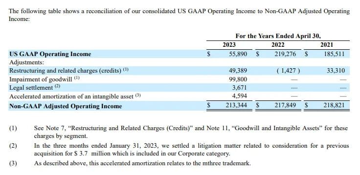
Heathers points out that, because Wiley is a public company, certain of its business records are required to be public, and he found this:

Heathers explains:

‘Legal settlement’ is exactly what it sounds like, and the footnote description is ‘a litigation matter related to consideration for a previous acquisition’.

The shorthand is: their own shareholders sued them. They said they were going to, and did. . . .

This is not uncommon . . . Any large public company in business for long enough has seen a suit or two like this. . . . Generally, they settle. . . . this is noticeably more expensive than running a full-scale proactive research integrity program.

And here’s the kicker:

For 3.7M, you could have the world. I [Heathers] am quite confident in saying: I could run that as the operating budget of a fraud mitigation unit for multiple years, and drop the amount of nonsense by . . . maybe two-thirds, three-quarters? within that time.

All right, then!

This is not new to Wiley

Just one thing. This is not new. Wiley’s been in the lucrative science-fraud business for awhile. Recall this story from 2011, “Wiley Wegman chutzpah update: Now you too can buy a selection of garbled Wikipedia articles, for a mere $1400-$2800 per year!”

But, yeah, the Hindawi business sounds a lot worse. When Wiley was conned by a formerly respected academic into republishing Wikipedia content and charging money for it, that was just a one-time breach in editorial standards. The Hindawi story seems like something else entirely. On the other hand, when it comes to fraudulent publishing, they had some track record.

Adversarial journalism

Heathers writes:

There absolutely IS adversarial journalism in academia/research/science/etc. Science Magazine, Undark, Vox, etc. have all published great pieces on this.

Ahhhh, Undark Magazine . . . that brings up memories. A few years ago, Undark published a terrible article, misrepresenting a scientific story in which I’d been involved. That was adversarial journalism in the worst sense, in that the journalists were coming in with an agenda and using it to distort and slam anyone who disagreed with it. See here for more on that story.

I’m not saying you shouldn’t trust anything in Undark just cos they ran that one bad article, any more than I’d un-recommend the books by Cochran just cos they were published by Wiley. I just thought it was funny that Heathers mentioned Undark in particular, given that my only experience with that magazine was so unpleasant.

What is “the definition of a professional career”?

I happened to come across this post from 2015 where I discussed a remark from a political journalist who advocated “some measure of accountability . . . which allows both that very bad teachers be fired and that very good ones can obtain greater pay and recognition. That’s the definition of a professional career track . . .”

What interested me there was not the question of how easy it should be to promote or fire teachers, but rather the idea that the risk of being fired is part of “the definition of a professional career track.”

OK, I’m not trying to take him literally. If you look up “professional” in the dictionary it says, “engaged in a profession that requires academic learning as preparation,” and if you look up “profession,” you get “a calling requiring specialized knowledge and often long and intensive academic preparation.” Obviously he didn’t literally mean that being fired is part of the definition, more that it’s a core or essential part of what being a professional is.

It was funny for me to see this because being a tenured professor is part of a professional career track, and we can’t be fired. Also, at a lot of universities there’s not much range for promotion either. On the other hand, I’d call journalism a profession too, and, unfortunately, journalists get fired all the time. Not just “very bad” journalists either. Journalists lose their jobs because of well-known economic factors leading to a decades-long decline in employment in that field.

I guess a more accurate way to put it is not that the risk of being fired is an essential part of a professional career track, but rather that this journalist thinks that this risk should be an essential part of any professional career track.

And I see where he’s coming from. I don’t want to be at risk of being fired–but there are lots of professors I know for whom, if they were fired, I’d be cool with that.

The thing I’m worried about is that whoever has the ability to do this firing will use this ability to extort things out of me or to retaliate at me. But I guess that’s where the “measure of accountability” comes in.

At this point I expect many of you will be groaning and saying that the vast majority of employees in this country can be fired for no reason at any time (“at-will employment,” as they call it) and I’m privileged to have a job where it’s really hard to fire me. To which I reply: I agree that I’m privileged, and not just in my job. I’m privileged in so many ways. Maybe more people should be privileged in this way!

But actually that’s not what I wanted to talk about here–we already covered most of this in our 2015 post and subsequent comment thread.

Here’s my question for you

Rather, I wanted to ask, from scratch, the question posed by the title of this post: What is “the definition of a professional career”?

The traditional definition, requiring academic learning, covers a lot. Doctors, lawyers, college professors all require long and intensive academic preparation. Physical therapists, too, and physical therapists do seem much more professional than they did thirty years ago. It also seems to me that professionalism involves some sort of standardization: a job category being more “professional” is often associated with a low variance, not necessarily in abilities but in how they comport themselves. When you go to a doctor or a dentist, they always act like doctors or dentists. Lawyers too, to some extent. Maybe K-12 teachers, not so much. K-12 teachers require academic learning but not so much as those other professions.

What about getting fired? Things have changed. Back in the day, doctors were mostly self-employed. Now I imagine they’re mostly employees. So I guess they can get fired. When you’re self-employed you can’t get fired but you can go out of business.

There’s also the distinction between the professions and the trades. For some reason, people always seem to want to bring up plumbers. To be a plumber you need training, but it’s not academic training. I guess you’d be a better plumber if you took a few physics classes, in the same way that it’s probably a good idea that pre-med students have to learn a bunch of biology. Architect is a profession because architectural training is academic, or because it’s traditionally an upper-middle-class job rather than a lower-middle-class job? And then there are lots of jobs that require little or no special training at all, but they require some skills or competence, like carrying boxes or caring for kids or elders. These sorts of jobs could become professionalized too, which is either a good thing or a bad thing, depending on how you think about it.

And then there’s journalism, and writing more generally. Traditionally no barriers to entry and a path forward for lots of people to make their mark, from Jim Thompson and Carl Bernstein on down: some of these people went to college and some didn’t–going to college is a great thing, you can learn a lot, even if it’s not giving you job qualifications–and even in later decades when more and more journalists were college graduates, it’s not like it was required.

I remember a bunch of years ago there were some political scientists writing about the professionalization of state legislators. In that context, “professional” meant that being a legislator was a full-time job, or close to it, with a good salary and some staff. In this case, professionalism had nothing to do with academic qualifications; it was being used in the same way as we talk about a “professional” athlete. A professional athlete makes a living from it; a semi-pro gets paid but needs some other job; an amateur does it just for fun.

So in a conversation about the so-called gig economy (speaking of journalists), being a professional means that you have a steady job that pays reasonably well. If you work at a nice restaurant, you can be a professional waitress. In that sense, I guess that many of my favorite novelists are not professional writers; they need to hold down other jobs such as teaching at universities. In which case they are professionals, but not at the task that uses their best talents.

P.S. Academic tenure only came up briefly in this post, but several people brought it up in the discussion. For those of you interested in my thoughts on the matter, I’ll point you to these two posts from 2011:

The “cushy life” of a University of Illinois sociology professor

Looking for a purpose in life: Update on that underworked and overpaid sociologist whose “main task as a university professor was self-cultivation”

The Pick-the-Winner-Picker Heuristic: Preference for Categorically Correct Forecasts

A couple years ago, Jay Naborn wrote:

I am studying people’s preference for categorically correct forecasts (such as getting the winner of a sports game right) over error-minimizing ones (such as getting close on the margin). We have experimental evidence of this, why it happens, etc.

What I would be interested in doing is demonstrating that this preference is/can be a mistake. To do so, it would be nice to show that doing well in terms of minimizing continuous error is a better predictor of future winner-picking than is doing well in terms of winner-picking. I am curious if you have any leads as to some existing dataset that would be helpful here, or some simulation/modeling strategy that may work.

I replied that, yes, this relates to a point we made here.

Recently Naborn followed up:

The blog post you sent (and a couple others of yours) were very informative for our background thinking. My work (with Jonathan Bogard) forecast evaluation is now published at the Journal of Marketing Research.

And here’s the abstract:

People routinely make decisions based on predictions made by others (e.g., political pundits, market analysts), so it is in their best interest to identify high-quality forecasts. Experts characterize good forecasting as minimization of continuous error (i.e., predictions close to the eventual outcome). By contrast, the present work reveals that laypeople typically see good forecasts as those that correctly predict an event’s categorical outcome (e.g., the winning team). Using within-subjects, between-subjects, and incentive-compatible designs, fifteen studies demonstrate this “pick-the-winner-picker heuristic” as well as its psychological mechanism: People evaluate forecasts by assigning separate weights to (a) categorical correctness and (b) continuous error minimization, depending on the overall importance of the categorical and continuous dimensions for that situation. Thus, in the common case when the categorical dimension matters most (e.g., sports contests), people prize forecasts that accurately predicted the categorical outcome (e.g., the winner, not the margin of victory). However, when the categorical dimension’s stakes are experimentally reduced, an attenuation is observed. While this describes how people typically evaluate forecasts, crucially, a dimension’s importance is not necessarily related to its diagnosticity of forecaster skill or reliability. Accordingly, the pick-the-winner-picker heuristic may constitute a normative mistake, while framing manipulations help debias judgments.

Interesting. It’s good to see research on this topic.

An economist writes: “the fulminations over the #1 pick seem overheated to me.”

Jonathan Falk writes:

I [Falk] am always amazed at the amount of (digital) ink spilled on the perverse incentives involved in taking to get the #1 draft pick. The current local woes of the Giants and Jets obviously contribute a lot to these discussions, but they happen all the time. As an economist, it’s clear to me that the value of a draft pick is the incremental value, not the absolute value. I’m completely aware that the upper tails of distributions have much more dispersion than the center, or even the 80th-90th percentile does, but the fulminations over the #1 pick still seem overheated to me.

First, of course, is the fact that assessment is made with error, and there are plenty of #1 busts in every sport. #2s can be busts as well, of course, but that merely lowers the expected difference between #1 and #2 as the true value of both is attenuated towards 0 — #1 loses more.

Second, there is the issue of team fit. Greatness is a vector, not a number, and if the teams ahead of you in draft order need something else, you still stand a chance of getting the player optimized for your needs. Going the other way, of course, is that higher draft picks absolutely lower the number of teams that can steal your guy.

Third, teams are… teams. One person can only contribute so much. So the relevant assessment is now how much better A is than B, but how much the addition of A versus the addition of B will change the prospects of your team — which I think is pretty obviously a lower difference, though I guess your rationale for voting runs in the other direction — you ought to judge a small incremental addition by the gigantic difference between winning a championship or not.

Fourth, more narrowly economic, every incrementally pick costs more. I don’t think that effect is huge in the context of overall payrolls, but isn’t that then another anomaly? If #1 picks are so dramatically better than, say, #5 picks, why aren’t they paid multiples more?

I don’t really have anything to say here, because I have no sense of how much teams are paying for #1 or #2 picks. I do remember a couple years ago that everyone was talking bout Wemby, but basketball’s different than football because there are only 5 players on the court, so one player can make more of a difference.

The case of Wemby makes me think that one way this could be studied would be to compare different years. In some years there is a clear consensus #1 pick, other years not.

A study is retracted after it turns out that its authors were misrepresented as “third-party experts” even though they were actually paid by the company?

Gur Huberman points to this news article:

A Study Is Retracted, Renewing Concerns About the Weedkiller Roundup

Problems with a 25-year-old landmark paper on the safety of Roundup’s active ingredient, glyphosate, have led to calls for the E.P.A. to reassess the widely used chemical.

In 2000, a landmark study claimed to set the record straight on glyphosate, a contentious weedkiller used on hundreds of millions of acres of farmland. The paper found that the chemical, the active ingredient in Roundup, wasn’t a human health risk despite evidence of a cancer link.

Last month, the study was retracted by the scientific journal that published it a quarter century ago . . .

The 2000 paper, a scientific review conducted by three independent scientists, was for decades cited by other researchers as evidence of Roundup’s safety. It became the cornerstone of regulations that deemed the weedkiller safe.

But since then, emails uncovered as part of lawsuits against the weedkiller’s manufacturer, Monsanto, have shown that the company’s scientists played a significant role in conceiving and writing the study.

Oh, what was that significant role?

Monsanto employees praised each other for their “hard work” on the paper, which included data collection, writing and review. One Monsanto employee expressed hope that the study would become “‘the’ reference on Roundup and glyphosate safety.” . . .

In retracting the study last month, the journal, Regulatory Toxicology and Pharmacology, cited “serious ethical concerns regarding the independence and accountability of the authors.” Martin van den Berg, the journal’s editor in chief, said the paper had based its conclusions largely on unpublished studies by Monsanto. . . . There was no disclosure of a conflict of interest on the part of the authors beyond a mention in the acknowledgments that Monsanto had provided scientific support.

There seems to be some controversy about the safety of this pesticide:

Dr. Philip J. Landrigan, who is a pediatrician and epidemiologist and the director of the Program in Global Public Health at Boston College . . . recently chaired an advisory committee for a global glyphosate study that found that even low doses of glyphosate-based herbicides caused leukemia in rats. . . .

Laboratory tests first flagged potential risks posed by exposure to glyphosate as far back as the early 1980s, and soon after, studies of Midwestern farmers exposed to herbicides started to show an increase in certain cancers. A U.S.-backed effort to eradicate coca fields in Colombia by spraying glyphosate from planes onto hundreds of thousands of acres of cropland led to widespread reports of illnesses among residents.

The 2000 paper declaring glyphosate safe was published against that backdrop. . . .

Bayer has paid out more than $10 billion to settle approximately 100,000 Roundup claims . . .

And then there’s the bigger picture:

The retraction points to a wider problem of research secretly funded by industries like tobacco and lead, said David Rosner, co-director of the Center for the History and Ethics of Public Health at Columbia University. “Shading the science to favor the corporate interest,” he said, was likely “the rule rather than the exception.” Journals needed to “press scientists more forcefully to identify conflicts of interest,” he said. “Huge financial interests are at stake.”

The most disturbing thing in the linked emails was that the Monsanto people referred to the authors of that paper as “third party experts” and as “independent experts.”

But if they were paid by Monsanto, then it doesn’t seem accurate to characterize them as “third party” or “independent” experts.

The research article appeared in 2000. The emails were released in 2017 in the process of a lawsuit. The article was retracted in 2025 (although the official publication date of the retraction is February, 2026, i.e., a month after the writing of this post).

I don’t know what to think about all this. On one hand, how much can you trust research on a controversial topic that was written, funded, and reviewed by one of the parties to the controversy? They do say this in the paper, “In this effort, the authors have had the cooperation of Monsanto Company that has provided complete access to its database of studies and other documentation,” but it sounds like Monsanto provided more than data access.

I guess I could try to read the original article . . . .OK, let’s take a look:

The paper goes into details on three studies from 1988, 1991, and 1992 of oral doses in rats over 10 or 15 days. Then it looks like there was another study from 1973 on oral doses in rats for 15 days, and then three studies of skin exposure from 1983 and 1991, two on monkeys and one on humans. Then there’s a mouse study from 1992, rat studies from 1987 and 1992, a dog study from 1985, a rat study from 1979, a mouse study from 1983, a rat study from 1981, . . . ok, I’m getting tired now. There’s not really much for me to chew on here as a statistician. It does seem that belief in these results is going to boil down to your trust in the research team, and so the undisclosed conflicts of interest are a big deal.

On the other hand . . . I’ve done research funded by Novartis–they paid my colleagues and they paid me directly too. We published a paper based on that work–two of the authors were Novartis employees and two of the other authors had worked for me at the time (more precisely, they’d worked at Columbia under my supervision). That project used Novartis data, but it was a little different from the above-discussed Roundup article in that its purpose was methods rather than policy.

Also I did some consulting for Monsanto at one point, I think! I can’t remember the details, I think I was on the scientific advisory board of some company that was doing some agricultural stuff, I went to one of their meetings and then I stopped hearing from them, actually I can’t even remember if they paid me. So I’m not gonna get on my high horse and denounce industry-funded or pharma-funded research in general terms.

“Making Your Research Free May Cost You”

Stephanie Lee writes:

Stephanie Rolin, a mental-health services researcher, found out last month that a journal had accepted her latest paper for publication. But there was an asterisk. Community Mental Health Journal was requiring her to fork over about $4,400 — a fee that she hadn’t budgeted for, and one she says she cannot afford. . . .

Most studies appear in paywalled journals, and critics have long contended that those paywalls enrich publishers while gatekeeping taxpayers from the research they fund. The NIH has been pushing for more openness in the ecosystem into which it pours nearly $48 billion annually, and its biggest move yet took effect on July 1. Under a policy that was approved by the Biden administration to take effect at the end of 2025, and moved up six months by the Trump administration, all agency-funded research must now be made freely and immediately available. The previous policy had allowed papers to stay paywalled for up to a year.

But since July 1, some publishers have only given researchers one way to comply with the NIH’s mandate: paying fees that were previously optional. In a year when federal funding has been exceptionally unreliable, scientists say they are stressed about spending thousands of grant dollars on unexpected and questionable open-access charges.

Things don’t have to be this way, open-science experts say: These fees are imposed entirely by publishers. The most prominent examples are Springer Nature and Elsevier, for-profit enterprises that generate billions in revenue. . . .

When Rolin submitted to Community Mental Health Journal earlier this year, she expected the process to go as it had when she’d published in its pages before. At the time, Springer Nature — which sets policies for the 3,000-plus journals under its umbrella — gave NIH-funded authors a “hybrid” of two choices. They could pay an open-access fee to make their study available right away. Or, for free, they could put their paper behind the journal’s paywall while preparing a second copy that was identical save for formatting changes and copy edits. Within 12 months of journal publication, this author’s version would become openly available on a federal database called PubMed Central, in line with a 2008-era NIH requirement. . . .

In late July, Community Mental Health Journal hit Rolin with a $4,390 bill for article-processing charges. Springer Nature’s website now explains that publishing behind a paywall is “not a viable option” for authors like her because it “conflicts with immediate public access policies, such as NIH’s policy.” . . .

Rolin said she’d been aware that the NIH policy was forthcoming, but was surprised by Springer Nature’s hard-line interpretation. Similarly, Elsevier’s terms and conditions for putting studies on PubMed Central list options that involve either author-paid fees or delayed embargoes that wouldn’t comply with the NIH’s mandate. A page describing how NIH-funded authors can “comply with NIH’s public access requirements” has been deleted. . . .

Not every publisher is responding in kind. The JAMA journals, published by the American Medical Association, say that immediately after publication, authors can post their accepted manuscript in a repository of their choice. . . .

But Springer Nature and Elsevier aren’t the only ones reacting to the NIH’s mandate this way. Melanie J. Scott, an associate professor of surgery at the University of Pittsburgh, had a paper accepted in August by the Journal of Leukocyte Biology, which is published by the Society for Leukocyte Biology and Oxford University Press. . . .

In the meantime, researchers will have to figure out how to foot the bill. . . .

Now I’m wondering exactly what is the government policy. I’d think it would be fine to post the paper on a preprint server such as Arxiv, then it doesn’t matter what’s happening with the journals, right?

The funny thing is, this happened to me just the other day, with this article, I think it was, which is indeed published at a Springer journal. Fortunately for me, this research was not NIH-funded so I did not need to pay, nor did I need to withdraw my submission from the journal. I can’t remember how much they wanted to charge me because I was never going to pay. Maybe $2K? And Theory and Society is not a major journal! I like Theory and Society–I’ve published two papers there in the past year–; I’m just saying that it’s wack to ask someone to pay $2K to publish there.

P.S. It’s good to see a government policy that was pushed by both the Biden and Trump administrations so we can talk about it without getting into a political tangle.

Here’s a story from Australia: There were so many problems with the survey that the government didn’t release the data.

From the Australian Bureau of Statistics:

On 17 July 2025 the Australian Bureau of Statistics (ABS) announced that it will not release statistics from the 2023-24 Survey of Income and Housing (SIH), noting that the data did not meet the ABS’ high standards for official statistics.

Wow!

Here’s the background:

The ABS has conducted surveys of household income in various forms since 1974, and the SIH has been conducted in its current form since 2003-04. It gathers data on household income sources and amounts, net worth, housing situations, and both household and personal characteristics.

While SIH has been conducted on a 2 yearly basis since 2003-04, the last annual results were released from the 2019-20 cycle. The scheduled 2021-22 cycle was cancelled in December 2021 due to disruption and statistical impacts associated with the COVID-19 pandemic. . . .

Across its survey program the ABS evolves its collection approach, wherever possible, to improve efficiency and reduce cost, reduce demands on the Australian public to provide their data, improve respondent experiences and take advantage of methodological and technological innovations. While these innovations are not always visible to data users, they are critical to maintaining the quality of official statistics and have been a feature of the SIH program since its inception.

They continue:

Given an increasing public preference for digital engagement, ABS made changes to the SIH 2023-24 sample design with the intention of delivering high quality data while making it easier for households to complete the survey. A new approach was implemented whereby the sample was divided into two groups to reduce any potential statistical impact arising from households not responding to a digital survey.

One group was randomly selected for ‘self-enumeration only’ using a digital (web or phone) approach, with no interview follow-up of non-responding households. In the second group, those households that did not complete a web or phone interview were assigned for field follow-up by an interviewer. This sample design allows the ABS to apply statistical adjustments to address potential under-representation of groups that were less likely to provide a digital survey response.

Unfortunately, when implemented, system and business process limitations resulted in some households in the second group not receiving the field follow-up required to support this design. This left the survey results open to bias arising from systematic differences between those who responded to the survey and those who did not. . . .

The ABS had planned to process SIH 2023-24 data progressively from the commencement of data collection, allowing an early assessment of data quality. Unfortunately, initial data extraction was significantly delayed by system problems, which in turn delayed the commencement of data processing. SIH 2023-24 data collection ceased on 30 June 2024. The inability to transfer the collected data from the data collection system to the statistical compilation system was not resolved until December 2024. . . . Detailed, aggregated data comparisons were made against previous iterations of the SIH, the Australian System of National Accounts (ASNA), the Person Level Integrated Data Asset (PLIDA), and non-ABS sources such as the Household, Income and Labour Dynamics (HILDA) survey.

These assessments identified inconsistencies, including:

Estimates of personal and household income were much lower than expected when compared to previous iterations of SIH or information in the National Accounts and other sources.
Aggregate liabilities and loan values were lower than expected, and exhibited lower coverage compared to the National Accounts than previous SIH cycles.
An observed decrease in superannuation income since SIH 2019-20 was not consistent with other sources and population trends.
Falls in outstanding mortgage values since SIH 2019-20 were also inconsistent with trends observed in other sources.

So:

Taken together, these results suggested the SIH 2023-24 results were not fit-for-purpose and led ABS to initiate an internal Quality Incident Response Plan (QIRP) process. . . .

Following review, the QIRP process confirmed that the observed data quality issues stemmed from two key statistical limitations discussed above, namely:

• A pattern of survey non-response that reduced the representativeness of the results.

• Pervasive question level non-response and response error, largely caused by ‘skippable’ questions in the survey form.

The QIRP panel found that the combined effect of these errors rendered the data unsuitable for its intended purpose.

That’s a big step. The report discusses the plans of the Australian Bureau of Statistics for this survey going forward.

The internet of poop

This is a funny story.

Who are these customers who would pay $600 + $6.99/month to have toilet cam photos uploaded to a consumer-products company?

I mean, I get it that Google’s grabbing all sorts of information on me right now, but at least I’m not directly paying for it. Are there really people who’d shell out all this money to share their poop-cam data?

I guess maybe the same sorts of people who fall for the government’s junk science, or who buy the supplements advertised by Dr. Oz, Andrew Huberman, etc. Maybe they upload their poop photos after taking their Stanford-recommended cold showers.

A year of this service would cost $683.88. For this price you could afford 440 Jamaican beef patties, one-tenth of a paper in Nature Communications, or 1/27th of an invitation to a conference featuring Grover Norquist, Gray Davis, and a rabbi.

I’d take the Jamaican beef patties . . . but maybe after eating 440 of them I’d actually need the poop cam!