Andy Wheeler writes:
I think this back and forth may be of interest to you and your readers.
There was a published paper attributing very large increases in homicides in Philadelphia to the policies by progressive prosecutor Larry Krasner (+70 homicides a year!). A group of researchers then published a thorough critique, going through different potential variants of data and models, showing that quite a few reasonable variants estimate reduced homicides (with standard errors often covering 0):
– Hogan original paper,
– Kaplan et al critique
– Hogan response
– my writeupI know those posts are a lot of weeds to dig into, but they touch on quite a few topics that are recurring themes for your blog—many researcher degrees of freedom in synthetic control designs, published papers getting more deference (the Kaplan critique was rejected by the same journal), a researcher not sharing data/code and using that obfuscation as a shield in response to critics (e.g. your replication data is bad so your critique is invalid).
I took a look, and . . . I think this use of synthetic control analysis is not good. I pretty much agree with Wheeler, except that I’d go further than he does in my criticism. He says the synthetic control analysis in the study in question has data issues and problems with forking paths; I’d say that even without any issues of data and forking paths (for example, had the analysis been preregistered), I still would not like it.
Overview
Before getting to the statistical details, let’s review the substantive context. From the original article by Hogan:
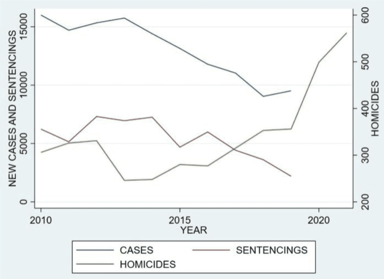
De-prosecution is a policy not to prosecute certain criminal offenses, regardless of whether the crimes were committed. The research question here is whether the application of a de-prosecution policy has an effect on the number of homicides for large cities in the United States. Philadelphia presents a natural experiment to examine this question. During 2010–2014, the Philadelphia District Attorney’s Office maintained a consistent and robust number of prosecutions and sentencings. During 2015–2019, the office engaged in a systematic policy of de-prosecution for both felony and misdemeanor cases. . . . Philadelphia experienced a concurrent and historically large increase in homicides.
I would phrase this slightly differently. Rather than saying, “Here’s a general research question, and we have a natural experiment to learn about it,” I’d prefer the formulation, “Here’s something interesting that happened, and let’s try to understand it.”
It’s tricky. On one hand, yes, one of the major reasons for arguing about the effect of Philadelphia’s policy on Philadelphia is to get a sense of the effect of similar policies there and elsewhere in the future. On the other hand, Hogan’s paper is very much focused on Philadelphia between 2015 and 2019. It’s not constructed as an observational study of any general question about policies. Yes, he pulls out some other cities that he characterizes as having different general policies, but there’s no attempt to fully involve those other cities in the analysis; they’re just used as comparisons to Philadelphia. So ultimately it’s an N=1 analysis—a quantitative case study—and I think the title of the paper should respect that.
Following our “Why ask why” framework, the Philadelphia story is an interesting data point motivating a more systematic study of the effect of prosecution policies and crime. For now we have this comparison of the treatment case of Philadelphia to the control of 100 other U.S. cities.
Here are some of the data. From Wheeler (2023), here’s a comparison of trends in homicide rates in Philadelphia to three other cities:
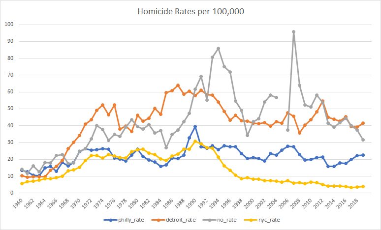
Wheeler chooses these particular three comparison cities because they were the ones that were picked by the algorithm used by Hogan (2022). Hogan’s analysis compares Philadelphia from 2015-2019 to a weighted average of Detroit, New Orleans, and New York during those years, with those cities chosen because their weighted average lined up to that of Philadelphia during the years 2010-2014. From Hogan:
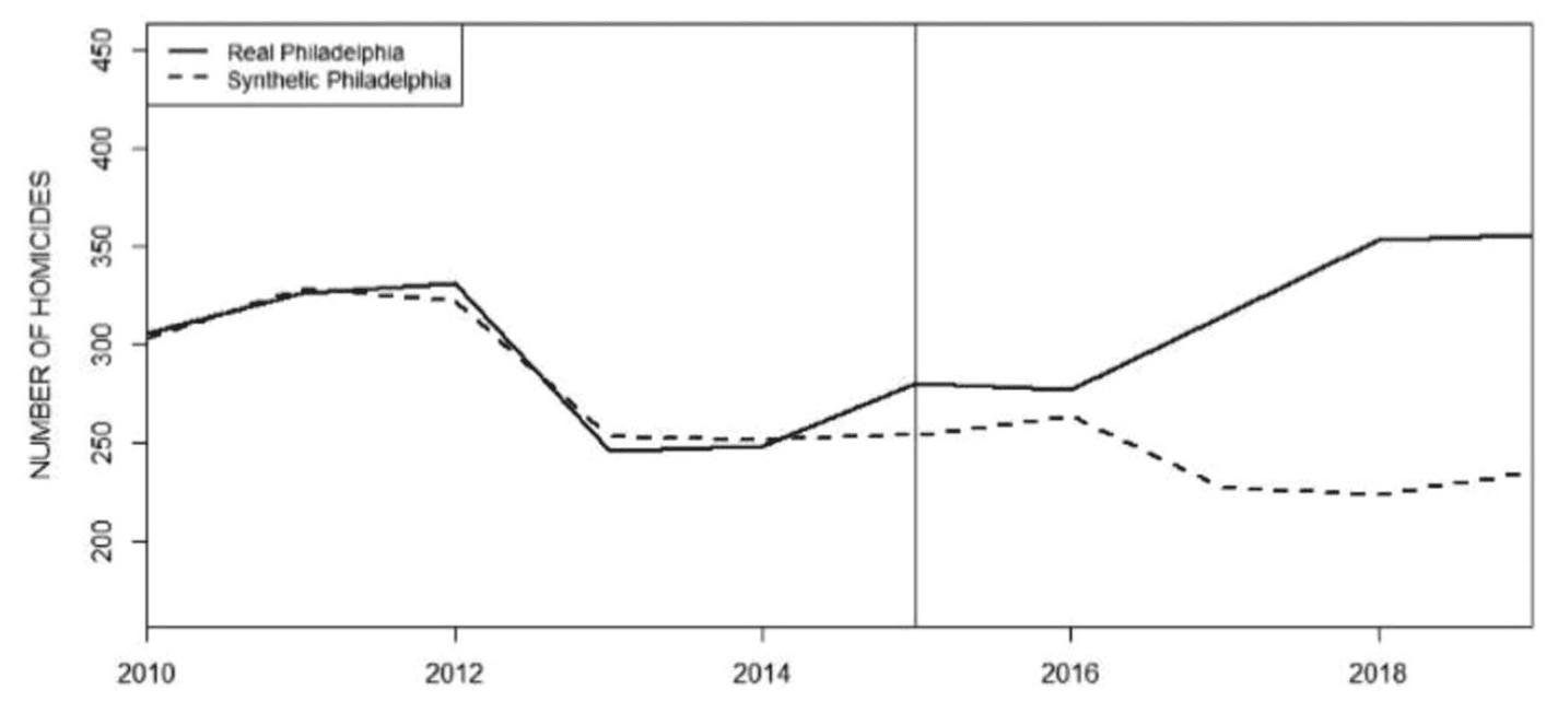
As Wheeler says, it’s kinda goofy for Hogan to line these up using homicide count rather than homicide rates . . . I’ll have more to say in a bit regarding this use of synthetic control analysis. For now, let me just note that the general pattern in Wheeler’s longer time series graph is consistent with Hogan’s story: Philadelphia’s homicide rate moved up and down over the decades, in vaguely similar ways to the other cities (increasing throughout the 1960s, slightly declining in the mid-1970s, rising again in the late-1980s, then gradually declining since 1990), but then steadily increasing from 2014 onward. I’d like to see more cities on this graph (natural comparisons to Philadelphia would be other Rust Belt cities such as Baltimore and Cleveland. Also, hey, why not show a mix of other large cities such as LA, Chicago, Houston, Miami, etc.) but this is what I’ve got here. Also it’s annoying that the above graphs stop in 2019. Hogan does have this graph just for Philadelphia that goes to 2021, though:
As you can see, the increase in homicides in Philadelphia continued, which is again consistent with Hogan’s story. Why only use data up to 2019 in the analyses? Hogan writes:
The years 2020–2021 have been intentionally excluded from the analysis for two reasons. First, the AOPC and Sentencing Commission data for 2020 and 2021 were not yet available as of the writing of this article. Second, the 2020–2021 data may be viewed as aberrational because of the coronavirus pandemic and civil unrest related to the murder of George Floyd in Minnesota.
I’d still like to see the analysis including 2020 and 2021. The main analysis is the comparison of time series of homicide rates, and, for that, the AOPC and Sentencing Commission data would not be needed, right?
In any case, based on the graphs above, my overview is that, yeah, homicides went up a lot in Philadelphia since 2014, an increase that coincided with reduced prosecutions and which didn’t seem to be happening in other cities during this period. At least, so I think. I’d like to see the time series for the rates in the other 96 cities in the data as well, going from, say, 2000, all the way to 2021 (or to 2022 if homicide data from that year are now available).
I don’t have those 96 cities, but I did find this graph going up to 2000 from a different Wheeler post:

Ignore the shaded intervals; what I care about here is the data. (And, yeah, the graph should include zero, since it’s in the neighborhood.) There has been a national increase in homicides since 2014. Unfortunately, from this national trend line alone I can’t separate out Philadelphia and any other cities that might have instituted a de-prosecution strategy during this period.
So, my summary, based on reading all the articles and discussions linked above, is . . . I just can’t say! Philadelphia’s homicide rate went up since 2014 during the same period that it decreased prosecutions, and this was part of a national trend of increased homicides—but there’s no easy way given the directly available information to compare to other cities with and without that policy. This is not to say that Hogan is wrong about the policy impacts, just that I don’t see any clear comparisons here.
The synthetic controls analysis
Hogan and the others make comparisons, but the comparisons they make are to that weighted average of Detroit, New Orleans, and New York. The trouble is . . . that’s just 3 cities, and homicide rates can vary a lot from city to city. It just doesn’t make sense to throw away the other 96 cities in your data. The implied counterfactual is that if Philadelphia had continued post-2014 with its earlier sentencing policy, that its homicide rates would look like this weighted average of Detroit, New Orleans, and New York—but there’s no reason to expect that, as this averaging is chosen by lining up the homicide rates from 2010-2014 (actually the counts and populations, not the rates, but that doesn’t affect my general point so I’ll just talk about rates right now, as that’s what makes more sense).
And here’s the point: There’s no good reason to think that an average of three cities that give you numbers comparable to Philadelphia’s for the homicide rates in the five previous years will give you a reasonable counterfactual for trends in the next five years. To think there’s no mathematical reason we should expect the time series to work that way, nor do I see any substantive reason based on sociology or criminology or whatever to expect anything special from a weighted average of cities that is constructed to line up with Philadelphia’s numbers for those three years.
The other thing is that this weighted-average thing is not what I’d imagined when I first heard that this was a synthetic controls analysis.
My understanding of a synthetic controls analysis went like this. You want to compare Philadelphia to other cities, but there are no other cities that are just like Philadelphia, so you break up the city into neighborhoods and find comparable neighborhoods in other cities . . . and when you’re done you’ve created this composite “city,” using pieces of other cities, that functions as a pseudo-Philadelphia. In creating this composite, you use lots of neighborhood characteristics, not just matching on a single outcome variable. And then you do all of this with other cities in your treatment group (cities that followed a de-prosecution strategy).
The synthetic controls analysis here differed from what I was expecting in three ways:
1. It did not break up Philadelphia and the other cities into pieces, jigsaw-style. Instead, it formed a pseudo-Philadelphia by taking a weighted average of other cities. This is a much more limited approach, using much less information, and I don’t see it as creating a pseudo-Philadelphia in the full synthetic-controls sense.
2. It only used that one variable to match the cities, leading to concerns about comparability that Wheeler discusses.
3. It was only done for Philadelphia; that’s the N=1 problem.
Researcher degrees of freedom, forking paths, and how to think about them here
Wheeler points out many forking paths in Hogan’s analysis, lots of data-dependent decision rules in the coding and analysis. (One thing that’s come up before in other settings: At this point, you might ask how do we know that Hogan’s decisions were data-dependent, as this is a counterfactual statement involving the analyses he would’ve had done had the data been different. And my answer, as in previous cases, is that, given that the analysis was not pre-registered, we can only assume it is data-dependent. I say this partly because every non-preregistered analysis I’ve ever done has been in the context of the data, also because if all the data coding and analysis decisions had been made ahead of time (which is what been required for these decisions to not be data-dependent), then why not preregister? Finally let me emphasize that researcher degrees of freedom and forking paths do not represent criticisms of flaws of a study; they’re just a description of what was done, and in general I don’t think they’re a bad thing at all; indeed, almost all the papers I’ve ever published include many many data-dependent coding and decision rules.)
Given all the forking paths, we should not take Hogan’s claims of statistical significance at face value, and indeed the critics find that various alternative analyses can change the results.
In their criticism, Kaplan et al. say that reasonable alternative specifications can lead to null or even opposite results compared to what Hogan reported. I don’t know if I completely buy this—given that Philadelphia’s homicide rate increased so much since 2014, it seems hard for me to see how a reasonable estimate would find that its policy rate reduced the homicide rate.
To me, the real concern is with comparing Philadelphia to just three other cities. Forking paths are real, but I’d have this concern even if the analysis were identical and it had been preregistered. Preregister it, whatever, you’re still only comparing to three cities, and I’d like to see more.
Not junk science, just difficult science
As Wheeler implicitly says in his discussion, Hogan’s paper is not junk science—it’s not like those papers on beauty and sex ratio, or ovulation and voting, or air rage, himmicanes, ages ending in 9, or the rest of our gallery of wasted effort. Hogan and the others are studying real issues. The problem is that the data are observational, the data are sparse and highly variable; that is, the problem is hard. And it doesn’t help when researchers are under the impression that these real difficulties can be easily resolved using canned statistical identification techniques. In that aspect, we can draw an analogy to the notorious air-pollution-in-China paper. But this one’s even harder, in the following sense: The air-pollution-in-China paper included a graph with two screaming problems: an estimated life expectancy of 91 and an out-of-control nonlinear fitted curve. In contrast, the graphs in the Philadelphia-analysis paper all look reasonable enough. There’s nothing obviously wrong with the analysis, and the problem is a more subtle issue of the analysis not fully accounting for variation in the data.
This might be discussed in the papers somewhere, but another factor to consider is that gun homicides (which are most of all homicides) are a noisy measure of shootings. By that I mean that someone shoots someone, and sometimes that person dies and sometimes they don’t. So even if Philadelphia had an increase in homicides relative to other cities you would want to examine if that was from an increase in shootings (crime) or a decrease in ambulance response or doctor efficiency or plain bad luck (not crime).
Why would there be a decrease in ambulance response or doctor efficiency all of a sudden in Philadelphia? How would you take “plain bad luck” into account?
It’s more of a general point. Perhaps there was some funding change in 2016, or the start of a long-lasting strike by hospital workers, or whatever. I’m not saying those things happened but in general if the analysis doesn’t look it can’t eliminate other possible explanations.
As to the ‘bad luck’, you account for it at least in part by looking at shootings instead of murders. If shootings stayed at the same level but murders changed, you can assume (broadly speaking) that the level of crime didn’t change but there was some other factor at play. A source I found said that there were ~1300 shootings in Philadelphia in 2016. If 5% of those happened to fatal instead of not, that’s 65 murders versus not-murders.
I can’t access Hogan’s paper, but given that they’ve cited Abadie, Diamond and Hainmueller, I’m going to assume Hogan used a similar approach as those authors. For whatever reason, it’s a common result of the ADH-style Synthetic Control procedure that your synthetic control ends up being composed of the weighted average of only a handful of candidates, no matter how many different potential candidates you input. A few questions came to mind while reading through this post:
1) Why is it better to include more cities in the Synthetic Control? Is the argument that putting a weight of 0 on all the other cities is very unlikely to be the appropriate choice?
2) Why would the jigsaw approach be superior? Putting aside any potential data-quality issues, I would think that crime rates at the neighbourhood level would be more volatile than crime rates at the city level, and so finding comparable neighbourhoods would be as difficult as comparable cities
3) IIRC a common sanity-check for the Synthetic Control procedure is running something like a placebo test, where you pick a city that didn’t have the proposed policy implemented, and show that the crime rate in the generated synthetic control still closely follows the actual rate in the treatment period. Any thoughts on this?
FYI, the reason zero weights are common in ADH-style synthetic control is the constraint that the weights are positive. This is a non-smooth constraint and tends to lead to edge solutions much like a constraind on the l1-norm in lasso. This also has a regularizing effect and dropping the positivity constraint usually necessitates some form of regularization as in Dudchenko and Imbens.
To me, the Philly curve looks basically *constant* from 1970 to 2019 (with perhaps a blip around 1990). The small ups and downs are, of course, impactful to the victims. But it’s hard to believe any single policy can explain them. One or two mass events, triggered by emotion, drugs, bad luck, mental illness, etc… can cause almost all the variation we see.
Note: That’s all the opinion of a rank-amateur social scientist and statistician. Just giving the view of an “outsider”.
By chance, Propublica has a current story that mentions the Hogan paper: https://www.propublica.org/article/police-politicians-undermined-reform-prosecutors-chicago-philadelphia
Indeed.
I’ve read much about how crime is up because of police reluctance to enforce laws as a function of frustration from understaffing or calls for defunding, or fear of investigation, or indifference because criminals won’t be held accountable, etc.
The timing doesn’t necessarily exactly line up with this study in some senses (much of that discussion is focused on post George Floyd), but isolating a discrete cause-and-effect here related to one specific policy seems kind of unrealistic to me.
In Philly, it seems obvious that police reactions to the policies (due to contempt for Krasner among the police union and some of the rank and file) as a factor in crime rates couldn’t be realistically disaggregated from the direct effects of the policies in themselves.
It’s prolly worth noting that for all the certainty among political pundits that the DA in San Francisco was the “cause” of higher crimes rates when he was in office, the lack of reduction in crime once he was booted out might suggest otherwise.
One thing that really jumps out from the first graph (‘Homicide Rates’) is how much more variation you see in New Orleans compared to the other cites. Of course, this is not surprising as homicide is a rare event and the population of New Orleans is quite small compared to the other cities. I wonder how (if at all) the synthetic control approach deals with this?
Default synth does not, I have attempted some dumb not think about it very hard optimization for matching on a proper population weighted average, https://github.com/apwheele/Blog_Code/blob/master/Python/SynthEstimates/rate_synth.py, but did not turn out so well. And moved onto other things.
IMO using lasso regression is a better default than the Abadie estimator, but this problem still remains. And it may be just doing the larger panel Diff-In-Diff is a better approach, which is kind of more consistent with Gelman’s suggestion (minus the post before this one!)
Thanks for the response Andy. I checked your pages and it looks like you’re trying to do something with rates instead of counts? I don’t think that really gets at what I’m saying. Basically, with small populations you have a small sample problem with rare events. So even if you use rates (and it’s rates in the graph above), you’re going to see a lot more variability in the small populations (like New Orleans).
I haven’t really thought about this in terms of synthetic controls but it seems it could be problematic, you’re comparing Philly to something (or a weighted average that includes something) that is a very noisy measurement.
So agree the variance of small sample rates is a problem (I don’t want to spam here with posts, but if you look on my blog I have various posts on funnel graphs and monitoring time series trends for homicide data).
So traditional synth via some simplified text math is:
min { Y_t – sum(w*Y_c) }
Y_t is typically rates, Hogan uses counts. So with rates you could have a scenario:
Treated [ Controls ]
BigCity BigCity1 TinyCity2
Rate 40 20 60
Pop 1e6 1e6 1e5
Count 500 200 30
So weights here of 0.5 for each is fine when matching on weights. But the population weighted average is (200 + 60)/(1e6 + 1e5) = 24 per 100k. The estimator I was trying to write matched on the population weighted average, not the naive sum of the rates. But you are right in that it was not working well (and theoretically could still just give a bunch of tiny locations, but have a weighted average match still).
Another idea I had is that you have the traditional equation above, but add a penalty term (similar to Lasso), so say V_c = Variance(Y_c) (the variance of the rate). So something like:
min { Y_t – sum(w*Y_c) + lambda*sum(w*V_c) }
Probably the Bayesian folks on this blog have a smart way to do similarish things like that with error measurement models as well.
Unpopular opinion: Synthetic Controls are BOGUS
https://qbnets.wordpress.com/2022/08/17/why-i-think-synthetic-controls-are-bogus/
I recently studied the synthetic control method a bit. I agree that the assumption that one city behaves like a weighted average of the others is more than a little odd. I like the idea that there are latent factors that affect all units, but explaining basically all the variance as in the graph above looks like a case of overfitting to me*. I think other cities can tell us something about what happened in Philadelphia, but not everything. Maybe some kind of B/VAR setup with fundamentals would be a better idea than a weighted average.
*I could be convinced that it is not overfitting by showing that (blocked) k-fold cross validation with low k gives similar results all the time.
i’m surprised this is your first encounter with synthetic control. it’s been popular in economics causal inference for a while. it’s still viewed with suspicion and rarely gets into top journals (my view is that researchers see it as a “last resort”; it’s what you do when you have a very small number of treated units–usually 1— and no natural comparison group, which as you say is a very hard causal inference problem). i guess it’s still very marginal outside of economics. i do like your imagined version though, that sounds like it would be a very interesting estimator–someone should work on that!
“think there’s no mathematical reason we should expect the time series to work that way”
the theoretical work on synth mostly shows that it works when the time series have a latent factor structure. so basically synth will find states with a similar factor loadings. however, a recent paper by Jiafeng Chen (https://arxiv.org/abs/2202.08426) shows that synth has some nice properties without making assumptions about the time series, but only about the timing of the policy change
Sam:
In the above post it is clear that this was not my first encounter with synthetic control. It’s just that before I saw textbook-style examples that were clean and persuasive. The example discussed above was interesting because it was a crappy example of the method being used in the wild, as it were.
In their example, they don’t just have one treated unit; there were various cities with a range of crime-control strategies. If they just wanted to consider only Philadelphia compared to others, then fine, go for it. But it’s absolutely ridiculous to think that it will make sense to compare to a weighted average of three cities just based on the five past years. It just makes no sense, and all the theorems in the world won’t fix it; the theorems will just depend on conditions that don’t make sense in the application.
this *is* a textbook example of synthetic control, though. that’s why i assumed you hadn’t seen it before. your proposed definition of synthetic control sounds like a very interesting estimator, but i’ve never seen a paper using the term synthetic control that does anything like that
in Abadie and Gardeazabal (2003), the paper that introduced the synthetic control method, synthetic Basque is a weighted average of Catalonia (which received over 80% weight) and madrid.
in Abadie, Diamond and Hainmueller (2010), the paper that first introduced the software that made SC very popular, synthetic california is a weighted average of colorado, connecticut, montana, nevada, and utah
in Jones and Marinescu (2022), synthetic Alaska is a weighted average of Utah, Wyoming, Washington, Nevada, Montana, and Minnesota
i could go on…
the fact that synthetic control only puts positive weights on a small subset of states is due to the “simplex constraint” that the weights are non-negative and sum to 1 (i saw this point made by Ben-Michael, Feller and Rothstein (2011), because their “augmented synth” relaxes this assumption, allowing for negative weights)
perhaps there’s a different method that goes by the name synthetic control which i’m not aware of and for which these are not prototypical, but for the synthetic control method invented by Abadie and Gardeazabal and which the paper in question by Horgan uses, these are definitely textbook examples (they are literally used in textbooks! see here https://mixtape.scunning.com/10-synthetic_control)
Sam:
I heard of synthetic control a long time ago, I think before 2003 but I’m not sure. It was in a conversation with Rubin where he talked about breaking up a state into pieces and finding corresponding pieces from other states. The idea sounded cool. Then I saw the paper discussed in the above post and I was disappointed to see that a method that had been a creative solution to a challenging problem had been turned into a horrible “identification strategy” of the sort that has done so much damage in econometrics and policy analysis. I haven’t read the papers you mention in your comment, so I can’t really express any opinion on them. It’s possible that the method made sense in those particular examples; I don’t know.
Yes, at least as widely used “synthetic control” refers to the method introduced in those two papers.
Prior to the study of the Basque country, I think there are some uses of “synthetic control group” or “synthetic comparison group” to refer to the group created through matching. Most of the examples of the latter on Google Scholar seem to be from this researcher https://scholar.google.com/citations?user=mpYoI3AAAAAJ&hl=en&oi=sra.
i didn’t know Rubin had a connection to synthetic control–cool! Alberto Abadie was at MIT and Harvard around that time, so it makes sense that they would’ve been talking to each other. i’d be curious to hear of any examples of the Rubin method, if you’re aware of any
Andrew –
Very interesting post. Thanks.
As a long-time (former) Philly resident and an observer of Krasner, I really appreciate your discussion.
It’s my impression that pretty much concurrent with the years of this analysis there has been another development which is particularly relevant to Philly – related to the opioid crisis and Tranq, a very dangerous drug, the use of which has grown immensely, and about which I’ve read many articles that centered the growth on Philly (the Kensington neighborhood on particular).
I will acknowledge a tendency towards a pro-Krasner bias. But I also reflexively believe this kind of analysis is incredibly difficult to pull off. Seems to me that your idea of how this analysis would be better done looks like a no-brainer. And I have to wonder how any variety of other relevant confounders were treated. Just comparing across cities seems highly problematic to me. Not unlike how comparing across countries to try to evaluate COVID policies seemed highly dubious to me.
Joshua:
I know next to nothing about Philadelphia, but I do think the whole identification-strategies thing has led applied econometrics and policy analysis astray, by pushing researchers toward narrow methods rather than more open-ended scientific exploration.
I sympathize with the motivation for narrow methods. Econometricians have been warned for many years about specification searches and more recently about p-hacking, so there’s a real appeal to using a canned method that has desirable asymptotic properties and can’t be hacked. Unfortunately, (a) asymptotics don’t count for much if you’re doing state-level analysis and only using data from a few states, and (b) as discussed in the above post, even these seemingly fixed methods have many researcher degrees of freedom.
So, while I sympathize with the use of these procedures, I think they’re generally a bad idea because they detach researchers from fundamental principles of observational studies. I feel the same way about regression discontinuity analysis and instrumental variables. All these methods can be useful as part of a balanced diet but don’t always work so well when their users don’t keep their eyes on the ball.
Asymptotics. A new word!
Agree with all you wrote there.
In the name of doing what you can to get information while fully understanding the limitations… I was thinking of the Chetty research where he talks about the power of zip code level data for addressing these kinds of research questions. That seems to me to align with your post here.
https://www.cmc.edu/news/power-of-zip-code
Zooming out a bit, it seems like this question ultimately comes down to producing reasonable estimates of city-level homicide trends that can be used to make what is essentially a forecast. I can’t help but wonder if there is a clever application of multilevel modeling that would help mitigate some of the problems with the SCM approach. I have no idea what that approach would be but seems like it could at least provide a more principled approach to borrowing information from (more) comparison cities. That said, it also feels like the data are just not up to this task.