The Kappa Zoo: David Eubanks’s online monograph on rating models

David Eubanks writes:

My site is kappazoo.com, and it’s still a work in progress. I would rather have emailed after I had the new goodness-of-fit code done, but I saw that you’re doing a summer workshop (on Andrew’s blog) [editor: Modern Modeling Methods (M3)], so thought I’d mention it now.

It may be billed as a work in progress, but it’s a complete draft with no missing sections that provides a really nice overview of rating/crowdsourcing models. These are the models that dragged me into statistics, namely Bayesian rating models formulated as noisy measurement models. The first model of this kind that I or Eubanks could find was Phil Dawid and Allan Skene’s (1979) paper on rating.

Eubanks works through a great deal of workflow without calling it that. There are multiple model evaluation and comparison measures used and explained with connections to information-theoretic notions like entropy.

There’s a long discussion of Cohen’s kappa statistic, which is a commonly reported statistic measuring inter-rater agreement. As Eubanks notes, it doesn’t deliver on its promise of adequately measuring inter-rater agreement. The discussion is quite good here and complementary to the discussion from me and Becky Passonneau in our paper on rating in NLP, though our conclusions are the same.

I was surprised to see that Eubanks has a section comparing item-response theory (IRT) models with difficulty. I’ve been trying to convince people this is important for years. It took me around ten years to figure out how to move from Dawid and Skene’s IRT-0-like model to an IRT-1-like model, which we report in in our latest paper on crowdsourcing with difficulty parameters (which also works through a lot of Bayesian workflow in considering different models). I can’t identify what took so long—it seems so obvious to me now.

No, Bayes does not like Mayor Pete. (Pitfalls of using implied betting market odds to estimate electability.)

This one’s from 2019, but it’s worth reposting given recent interest in prediction markets.

The story starts with a post from economist Greg Mankiw, who wrote:

Who has the best chance of beating Donald Trump? A clue can be found using Bayes Theorem.

Here is the logic. Let A be the event that a candidate wins the general election, and B be the event that a candidate wins his or her party’s nomination. Predictit gives us the betting market’s view of P(A) and P(B). It is a safe assumption that P(B|A) = 1, that is, a candidate can win only if nominated. We can then use Bayes theorem to compute P(A|B), the probability that the candidate will win the general election conditional on being nominated.

So here are the results for P(A|B) as of now:

Buttigieg 0.80
Biden 0.77
O’Rourke 0.67
Sanders 0.65
Booker 0.60
Yang 0.60
Harris 0.57
Warren 0.44

That is, the betting markets suggest that Mayor Pete would be the strongest candidate if nominated, with Joe Biden close behind. (Of course, these numbers will bounce around as the prices in betting markets change.)

By the way, when I [Mankiw] did a similar calculation in 2006, Bayes liked Barack Obama.

I copied Mankiw’s post in its entirety, with the only change being that he wrote P(A / B) etc., and I changed the slash to the vertical bar, P(A|B). (Are there people who write conditioning using a slash rather than a vertical bar? I had no idea. P(A|B) is more standard, I believe. In the above post, Mankiw links to the wikipedia page which uses the P(A|B) notation. No big deal, it just seemed odd to me.)

Anyway, I think the above set of calculations is a great example for teaching conditional probability.

The next step is to push a bit: Do we really believe these numbers? There’s nothing wrong with the probability calculations, but I’m not sure we should be taking Predictit’s betting odds as actual win probabilities.

To start with, I looked at Mankiw’s list and wondered what Yang was doing on it. Yang’s a fringe candidate, right? I wrote my post in June, 2019, and Yang was polling at 0.8% on Real Clear Politics then. I went over to Predictit and it said you can buy a Yang contract for the Democratic nomination for the price of 9%. OK, sure, at 0.8% in the polls there’s room for improvement. But 9%??? Seems like a lot.

The next think I’m worried about, beyond bias in the online markets, is volatility.

Sure, Mankiw writes, “these numbers will bounce around as the prices in betting markets change,” but I think he’s not fully appreciating how noisy these numbers are!

Mankiw’s post is dated 27 Apr 2019. Predictit conveniently gives prices going back a few months, so I could do some Biden-Warren price comparisons of then to when I was writing my post:

27 Apr 12 Jun
Biden primary election 22 28
Biden general election 17 19
Warren primary election 9 19
Warren general election 4 13

Something weird was going on in April, when Biden’s price was 22 for the primary and 17 for the general election. This just can’t be right, and all I can conclude is that the betting markets here were thin enough that nobody was taking these numbers very seriously.

If you want to take the numbers as is, you’ll get the following:

27 Apr: Biden 17/22 = 0.77, Warren 4/9 = 0.44
12 Jun: Biden 19/28 = 0.68, Warren 13/19 = 0.68.

These numbers aren’t quite right, even if you take these betting markets seriously, because of rounding and the vig. If you add up all the prices on the “Who will win the 2020 Democratic presidential nomination?” page, you get something well over 100%. So you can’t directly interpret these prices as probabilities, even beyond the issues of bias and noise.

I discussed this with David Rothschild, who thinks a lot about elections and prediction markets (for example, here), and David responded as follows:

People ask me to compute this automatically on my blog, but I refrain, because it is so noisy this early. Here I compute the conditional probability range separately for Betfair and PredictIt, by diving the seller’s price of win / buyer’s price of nom & buyer’s price of win / seller’s price of nom. Betfair has advantage of being tighter by definition (PredictIt trades on the penny, but Betfair on the odds, which have more depth).

Here is a figure from an old paper I wrote with David Pennock about the 2012 election. As you can see, while informative, it can get quite noisy!

Anyway, my point here is not to criticize Mankiw but rather to thank him for putting out this fun example, and then to demonstrate how we can take it further by interrogating each step in the analysis. Which is how we do applied statistics in general.

P.S. In case you’re curious, based on the numbers when I wrote my post, where Biden’s implied electability is 19/28 = 0.68 and Warren’s is 13/19 = 0.68, we can look up Buttigieg. He was at 9/16 = 0.56, the least electable of the three. So, no, Bayes did not like Mayor Pete that day.

It’s a fun example, but when we look at the data more carefully, the original conclusion goes away.

Full day Stan tutorial at Modern Modeling Methods (M3) this summer in New York (22 June 2026)

This post is from Bob

Mitzi Morris and Bob Carpenter, two of Stan’s developers, will be presenting a tutorial on Stan and Bayesian data analysis aimed at psychometricians this summer.

Abstract

This workshop is a full day, hands-on introduction to Bayesian modeling and statistical inference using the probabilistic programming language Stan.

The course will be organized around the key properties of Bayesian statistical modeling for science, including the nature of uncertainty, modeling a generative process through a data generating distribution, modeling existing knowledge through a prior, and pushing uncertainty through inference. As we do this, we will show how Stan can be used to both code the models and perform statistical inference for quantities of interest, be they retrospective parameter estimates or prospective predictions or forecasts. We will concentrate on full Bayesian posterior inference, including a discussion of calibration, model checking for both prior and posterior inference, and model comparison with cross-validation. We will spend some time showing how some structural equation models (SEM) can be translated directly to Stan and will also introduce psychological models for educational testing, crowdsourcing, rating and ranking, and real-time decision processes.

This class will require a notebook computer with a network connection (Wifi will be available in the classroom). We will use the Stan Playground, which runs Stan in the browser, which we will pre-populate with models of interest. We will probably also break into R or Python at various points to demonstrate methods not yet supported by the Playground, such as the brms regression expression language.

Andrew on psychometrics

Andrew once told me that any model you could come up with was probably invented by a psychometrician 50 years ago (make that 60—he said it at least 10 years ago). I have evidence that he’s right form the project that drew me into Bayesian statistics—crowdsourcing. Andrew and Jennifer Hill helped me formulate a crowdsourcing model where raters give you noisy measurements of underlying categorical variables (e.g., they answer survey questions about whether a word in context is a noun, for example, to use something I was working on at the time). Turns out Phil Dawid and A.P. Skene published the same model in 1979 in one of the earlier applications of the expectation maximization (EM) algorithm and they used natural language data (drawn from medical records).

The rest of the conference

The rest of the program looks really great—it’s just the kind of applied wrestling with real data that I like.

Speaking of Jennifer Hill, she’s one of the keynote speakers at M3. Every talk of Jennifer’s I’ve attended has been great. You may know her as Andrew’s co-author on the regression books, which I cannot recommend highly enough if you’re interested in this kind of applied modeling.

Beyond the conference

You see the same kind of Bayesian modeling focus for real data at venues such as ISEC (international ecology conference to which I went to once just because I like these models and these kinds of conferences), StanCon (see you in Uppsala in August!), and GeoMed (which Mitzi attends). I’m sure there are more in other fields. I’m always disappointed that there’s almost nothing like these kinds of nitty-gritty applied papers at ISBA (Nagoya this summer) or BayesComp (somewhere next year). The conferences about Bayesian statistics or computing that I’ve been to have all been super theoretical.

MrPlew: Locally Equivalent Weights for Multilevel Regression and Poststratification

Ryan Giordano, Alice Cima, Jared Murray, Erin Hartman, and Avi Feller write:

Multilevel regression and poststratification (MrP) has become a workhorse method for estimating population quantities from non-probability surveys, and is the primary model-based alternative to traditional survey calibration weighting methods, such as raking. For simple linear regression models, MrP methods admit “equivalent weights”, allowing for direct comparisons between MrP and traditional calibration weighting. Such weights, however, have been unavailable for the most widely used MrP models, such as logistic regression. In this paper, we develop a natural generalization, “MrP locally equivalent weights” (MrPlew), which represent MrP as a weighting-style estimator that is locally equivalent to calibration weights near the observed responses.

Cool! This goes beyond my 2007 paper, Struggles with survey weighting and regression modeling (“for logistic regression, the poststratified estimate is no longer a weighted average of the data, even after controlling for the variance parameters in the model. However, we suspect that the model could be linearized, yielding approximate weights”) and our 2004 paper on dilution assays, in particular Section 5.2, “Equivalent weights for nonlinear models.” The funny thing is that I forgot about that 2004 paper when working on equivalent weights for MRP in the 2007 paper. Also, the 2004 method won’t work as is, because it’s designed to estimate sensitivity to individual data points, not to produce good weighted averages.

I say this not to try to claim credit for the method of Giordano et al., but rather the opposite, to emphasize that even though I’ve been thinking about equivalent weights in MRP for a long time, I haven’t yet succeeded in getting them to work in practice, so I’m very happy to see developments in this area.

One thing that came up with equivalent weights when we tried to apply them in practice is that sometimes the weights can be negative.

Negative weights can sometimes make statistical sense. The idea is that, depending on how the data line up in the regression model, sometimes if you pull one data point upward, it will cause the slope of the fitted line to change in such a way as to reduce the predicted mean value. This doesn’t sound right at first, but it can easily occur with poststratification when the population distribution of the predictors differs from the sample. Even if the negative weights can make sense in the estimation context, it still would seem kind of awkward to pass them along to the user.

The other thing that’s tricky is: What are the weights going to be used for? In the 2007 paper, the equivalent weights are set up to get the right answer for the estimate of the population mean, but presumably they’d be used for large subgroups too (for example, the average among men or women in the population). For more complicated estimates such as arise in small-area estimation or regression, you might want to use MRPW. Which is fine, but whatever it would take to get good weights for one of these purposes might not work best for the others.

Still, I remain interested in MRP locally equivalent weights of some sort, for two reasons:

1. We’re often doing MRP (or, more generally, RPP) anyway, so why not provide weights for other users of the survey that we’re analyzing?

2. Sometimes we’re called upon to provide weights for a public-facing survey, and the way we end up doing this is through an awkward and unsatisfying sequence of adjustment and smoothing steps (the “struggles” in “Struggles with survey weighting and regression modeling”). If we can do this using modeling and MRP, that could be a much more effective workflow, providing weights that are more stable and yield more accurate estimates of population quantities while also being more scientifically defensible and requiring fewer arbitrary choices.

Model-based weights will depend on some set of predictors X, variables that are observed in the sample and in the population (or, as necessary or appropriate, estimated from the population). One funny thing is that the weights will be mathematically a function of X, but the function itself will depend not just on sampling design, and not just on the distributions of X in the sample and population, but also on the outcome y that is being modeled. Different outcome variables will yield different sets of weights. At first this might seem disturbing, but upon reflection I think this dependence is a good thing. When it comes to weighting, the relative importance of the different variables in X will indeed depend on the outcome. Different variables are important for predicting public health risk factors than predicting how you will vote. That said, if you want some sort of omnibus weights, which you probably will want for a public survey, you can compute equivalent weights for each of a battery of outcomes and then average these weights to get a single set. That seems reasonable enough.

OK, back to Giordano et al., who continue:

This enables a suite of standard weighting diagnostics, including frequentist sampling variability, covariate balance, and subgroup contribution. We formally justify the use of MrPlew in these cases: we prove the MrPlew-based variance estimator is asymptotically equivalent to the infinitesimal jackknife for common exponential family models, and we introduce a novel class of model checks based on invariance to data perturbations that generalize covariate balance and subgroup contribution to nonlinear models. We further show that MrPlew can be computed easily using existing MCMC samples and provide open-source software to compute MrPlew using the output of standard software. We illustrate our approach for several canonical studies that use MrP, including via a logistic regression outcome model, showing that implied covariate balance can sometimes be worse for MrP than for raking. Given the ease of computing, we recommend making MrPlew a standard part of the MrP model interrogation workflow.

It makes sense that implied covariate balance can sometimes be worse for MRP than for raking. MRP is a smoothed version of raking, and unsmoothed raking can overfit. Or, in practice, you might rake on fewer variables so as to avoid overfitting. Multilevel regression gives you the freedom to include more predictors and interactions, secure in the understanding that the model will smooth the estimate and there will be less possibility for overfitting. In short, multilevel modeling–or, more generally, regularization–is a sort of safety net that can give us the security to construct better models, in the same way that a social safety net can give people the security to try new jobs, or for that matter in the same way that an actual safety net can give acrobats the security to perform more elaborate routines.

Where I want to go next is to be able to use these methods to construct weights for public surveys. I’m still not sure about all the steps that will take us there, but I continue to think it’s possible.

The new Giordano et al. paper is thoughtful and readable as well as having lots of math, statistical modeling, and real-data examples. I recommend you read it.

Jonah’s seminar tomorrow: “Bayesian Workflow and the Software That Shapes It”

This is Leo. Jonah Gabry (Stan developer, Andrew’s collaborator, etc.) is spending the whole month of May as a visiting professor here with us at the University of Trieste in Italy. Tomorrow, May 19th, in the De Finetti room at the University of Trieste, at  9 am NYC time (GMT-4), Jonah will give the following talk:

“Bayesian Workflow and the Software That Shapes It”

based on the upcoming book:  “Bayesian Workflow”.

For anyone local, you are welcome to come in person. Anyone else can join on Microsoft Teams (available here).

Alchemize: PyMC’s model to replace Stan/PyMC, etc. with an LLM

This post is from Bob

I’ll let Thomas Wiecki, who is one of the core PyMC devs and one of the partners at PyMC Labs, speak for himself here:

If you haven’t seen what people are doing with agentic AI, this is a good example. I’m really happy that Thomas and PyMC Labs are sharing their thoughts and initial tries at things like this as I think it has the potential to benefit everyone working on modeling.

If you want to see the basis of the agent’s instructions, check out the “skill” for PyMC that Chris Fonnesbeck wrote.

We’ve already batted this around a bit in email with Thomas, so I can summarize some talking points:

LLM-based chatbots are really good at translating. Compiling (or more technically correct, transpiling) a statistical model down to a language like Rust or C++ or JAX is a kind of translation.

You can start from PyMC’s execution trace, but you can also start with a model description. You could also start with something like Stan code.

The biggest bottleneck to deploying Bayesian models in my opinion is the inherent variance and unreliability of MCMC-based inference. Our workflow proposals are all about making sure this doesn’t go wrong. Wiecki’s point here is that we can have the bots go through the workflow. Iterating until the gradients and log densities match is a good example, but this could be extended to more parts of workflow.

The skills feel a lot like writing a textbook for a bot. I have no idea how hard or easy this is or how much it improves over the baseline. Jeremy Magland built a RAG-like helper for Stan that compressed the Stan Reference Manual down to 1K tokens for context (like a skill) and allowed it to search and import from the Stan User’s Guide, but never measured how much it improved over the baseline. It really feels like it should also have the Stan Functions Reference, BDA3, Regression and Other Stories, and the Bayesian Workflow book, as well.

Hopefully we’ll asymptote at writing a textbook sized set of skills and not have to write one per target model (that is, something like the Stan User’s Guide, Reference Manual, Functions Reference).

I’m curious as to whether it will eventually be able to make writing hard models easier. I’m thinking of efforts like epinow2, which involves a very large chunk of Stan code.

As the foundation models and chatbot tuning changes, there’s going to be an issue of regression testing and tuning for whatever the latest models are.

P.S. This effort explains how Thomas was able to create the huge posteriordb pull requests for PyMC (#320 and #319)!

P.P.S. The latest thing Claude (Opus 4.7) did that impressed me was generate the ess(MatrixXd, vector) function in summary.hpp. This function estimates effective sample size Stan style (discounting for R-hat > 1) on a ragged array of Markov chains. We have to generalize all the posterior analysis tools to deal with the new asynchronous parallel sampler). I had Stan’s ESS function and all the other functions I’d written for the ragged structures to give it as a guide. It’s very easy to code review that it matches Stan’s implementation for the new data structure. I only had to tweak the output a little bit for style.

“DC Conventional Wisdom Goes Down to Defeat in State after State”

Josh Marshall writes:

Elections are hard to predict. But even with that, some of the notional “surprises” we’re seeing [on Election Day, 2025] are less surprises than a measure of GOP dominance over current press narratives. People were looking for an upset in New Jersey. Nate Silver’s Silver Bulletin speculated that New Jersey might be moving toward becoming the next swing state. In fact, Rep. Mikie Sherrill (D) currently appears on track to crush Republican Jack Ciattarelli. A similar failure of conventional wisdom appears to be unfolding in the Virginia Attorney General’s race. A lot of D.C. insiders had convinced themselves that a controversy over some intemperate texts (not nothing but fairly close to it) had doomed his campaign. As recently as a couple days ago, betting markets (which are proxies for conventional wisdom) gave his opponent Jason Miyares 3-to-1 odds of victory. Jones now appears on his way to a clear though not resounding victory with a 3-to-4 percentage point margin.

Marshall continues:

These results aren’t terribly surprising. You’d expect Democratic gubernatorial candidates to do well in blue states in a climate where the Republican president is deeply unpopular. . . . The issue, again, is the power of Republican political narratives currently have over the elite political press. . . .

Maybe. But maybe it’s simpler than that; it’s just that journalists were reacting to the Republicans outperforming the polls in 2024.

In our election forecasts, we include terms to allow for the possibility of systematic state and national polling errors. There’s no perfect way to do this adjustment, and I’ve heard that some of the private polls in 2024 did better than the public polls that we and others were aggregating. The point is that there’s uncertainty.

Lots of people, even quantitatively-minded people, can’t seem to handle this uncertainty. For example, our 2024 forecast was criticized for not “communicating that a Trump landslide was a significant probability.” But the election was very close–nothing like a landslide at all!

The relevant point here is that people seem to be able to handle a point forecast (“Here’s who we think will win”) or complete uncertainty (“We know nothing at all”) but have difficulty with anything in between (“We’re pretty sure the election will be close, but it could go either way”). And I think what happens sometimes is that people take forecasts with uncertainty and place them in one of these two bins. For example, when we (and Nate, and others) gave our forecasts in 2024, the public–even some quantitatively-trained members of the public–were inclined to either treat our forecasts as deterministic (our forecast odds are 50/50 so we’re essentially predicting an exact tie) or as empty (our forecast odds are 50/50 so we’re making no predictions at all).

Now let’s get back to those 2025 elections. Democrats had comfortable polling leads in all these races, but pundits had been burned a year earlier, so a natural first step was to take the polling errors from 2024 and apply them to the 2025 polls. In the event, the polling errors were mostly in the other direction. On election eve, a reasonable forecast would be to say that the Democratic candidates were likely to win handily, they might win by even more than expected, or the races might have been close, with some Republican upsets not being out of the question. It’s hard for me to compare this to the conventional wisdom because that’s not written down in any one place.

Uncertainty is hard, especially given that people flip between thinking of forecasts as deterministic and thinking of forecasts as being completely uncertain. It’s related to the well-known challenge of producing wide-enough uncertainty intervals.

Survey Statistics: Blue Rose Research is (still) hiring !

As readers may know, I’m a survey statistician at Blue Rose Research. We survey the public to forecast elections and test political messages, used to advise Democrats. On this blog we’ve discussed our 2024 election retrospective and announced hiring (April 2025 and October 2025). And now we hiring again !

We are hiring a Machine Learning – Scientist (salary: $140k – $190k). This will be with our forecasting team, who track public opinion, forecast election results, develop resource allocation tools, and deliver polling analysis that clients rely on to set strategy. We’ve built a technical stack that enables cutting-edge statistical, machine learning, and engineering solutions.

Any additional roles we open up will be updated here. There’s an option to sign up for alerts for new roles via email if you’d like.

All positions are remote, with an option to be in person in New York City.

Please circulate and apply !

Expanding the Stan User’s Guide

This post is from Bob.

The Stan User’s Guide has been evolving organically along with the project. I’m writing this post for two reasons—to let you know what we’ve added lately and to encourage you to add your own chapters.

History

Initialy there was just one doc that included what is now the Reference Manual, Function sReference and CmdStan Manual. You can browse them all on the web or download pdfs from the Stan documentation web site.

Most of the topics grew up opportunistically from either things the team was interested in, new features we added to Stan, or just trying to cover the basics of the chapters of Bayesian Data Analysis and Data Analysis Using Regression and Multilevel/Hierarchical Models.

Recent additions

There have been some recent additions, including some from new faces:

There are also a metric ton of minor clarifications, fixes, and model examples, such as Mitzi Morris’s additional sufficient statistics optimizations and you can simply look at all the documentation pull requests.

The future is you

You can see from Franziska’s pull request, Abner’s PR, and Brynjólfur’s PR that we provide a lot of guidance and feedback. I found it super useful to write a lot of the documentation when I was learning statistics because I got feedback from Andrew Gelman, Ben Goodrich, Aki Vehtari, and Michael Betancourt, among others.

Some topics that would be nice to add

There is a lot to add to our existing discussions and you can see a lot of that in the pull request list on our documentation repository. There are also many topics that we don’t cover or don’t cover well. Off the top of my head, roughly ordered near the top according to my assessment of how impactful it would be to add.

  • causal inference using Rubin’s potential outcomes framework
  • Thompson sampling for reinforcement learning/bandits (sorry, Andrew!)
  • penalized complexity priors and the Besag-York-Molie II spatial model (working from Mitzi’s Morris’s case study)
  • Extreme value models
  • RNA-seq and DNA-seq composition models at the read level and k-mer level
  • Econometric models (I don’t even know what these are, but there are books)
  • Stationarity-constraining parameterizations of VAR models a la Sarah Heaps
  • Neural networks
  • A/B testing (ideally sequential)
  • spatio-temporal models along the lines of Leon Held’s survey
  • non-trivial examples of ODE models like Lotka-Volterra (my case study), SEIR (Elizaveta Semenova et al.’s case study) or even better, pharmacokinetic/pharmacodynamic (multiple case studies around Torsten), soil carbon (my very early case study, but there’s been much better work since)
  • Hilbert-space approximations to Gaussian processes (GPs)
  • PDE approximations to GPs
  • Fourier space analyses of GPs
  • N-gram language models
  • Plackett-Luce model for contest with more than two players (this can follow my case study for StanCon)

Some of those may already be mentioned in our doc, so sorry if you’ve already written something. Also, feel free to suggest more topics in the comments.

Should French pollsters be using Mister P?

An anonymous statistics student from France sends in the above plots (click twice to see big versions) and writes:

I’m trying to push French pollsters to start doing MRP.

I made a poll agregator and applied it to the last 100 days of the last five french presidential elections.

I did some smoothing using an algorithm from a paper of Aki Vehtari. It is Kalman-RTS with cross-validated levels of noises.

I tested it on some simulated data to confirm it is fitting properly.

I put the data and the code on my blog.

What I shared as “the data” is the smoothed result. I fitted it on the wikipedia pages of the french polls.

On the plots, the same parties (with changed names or fusions) are on the same position horizontally to allow comparisons.

I see some periodic movements in opinion that I think may be coming from a periodic non-response.
Also, the movements seem far too large to me. I can believe 10% increase for a candidate in five years, but not in less than 100 days.

The French polling industry is in profound need of reform. A fun fact: They allow themselves to change the final result by plus or minus one point based on the feelings of the person in charge of the poll. They call that the “pifomètre” or nosemeter. I heard about this in an interview with sociologist Hugo Touzet on his book, “Produire l’Opinion: Une Enquête Sur Le Travail Des Sondeurs.” I trust his descriptions of their methods since he has interviewed their workers.

I think MRP would allow the pollsters to do predictions for the legislative elections and municipal elections, which have been largely ignored because they are too difficult and expensive with quota sampling.

I know next to nothing about French polling, but, yeah, I do think they should be using Mister P (multilevel regression and poststratification; MRP).

P.S. Here’s a fun cranky post from this student.

The Bayesian Workflow book is coming!

We’re very excited about this book. It’s the result of several years of effort. You can pre-order from the publisher or from Amazon.

Here’s the book’s webpage, which includes the data and code for the book’s examples and case studies, of which there are many.

Here’s the table of contents:

Part 1: From Bayesian inference to Bayesian workflow
1. Bayesian theory and Bayesian practice
2. Statistical modeling and workflow
3. Computational tools
4. Introduction to workflow: Modeling performance on a multiple choice exam

Part 2: Statistical workflow
5. Building statistical models
6. Using simulations to capture uncertainty
7. Prediction, generalization, and causal inference
8. Visualizing and checking fitted models
9. Comparing and improving models
10. Statistical inference and scientific inference

Part 3: Computational workflow
11. Fitting statistical models
12. Diagnosing and fixing problems with fitting
13. Approximate algorithms and approximate models
14. Simulation-based calibration checking
15. Statistical modeling as software development

Part 4. Case studies
16. Coding a series of models: Simulated data of movie ratings
17. Prior specification for regression models: Reanalysis of a sleep study
18. Predictive model checking and comparison: Clinical trial
19. Building up to a hierarchical model: Coronavirus testing
20. Using a fitted model for decision analysis: Classification competition
21. Posterior predictive checking: Stochastic learning in dogs
22. Incremental development and testing: Black cat adoptions
23. Debugging a model: World Cup football
24. Leave-one-out cross validation model checking and comparison: Roaches
25. Model building and expansion: Golf putting
26. Model building with latent variables: Markov models for animal movement
27. Model building: Time-series decomposition for birthdays
28. Models for regression coefficients and variable selection: Student grades
29. Sampling problems with latent variables: No vehicles in the park
30. Challenge of multimodality: Differential equation for planetary motion
31. Simulation-based calibration checking in model development workflow

Appendices
A. Statistical and computational workflow for Bayesians and non-Bayesians
B. How to get the most out of Bayesian Data Analysis

One way to think of the book is that it’s all the things missing from BDA, like how to set up an informative prior, what to do when your computations aren’t converging, how to work through a series of models fit to the same data, how to design and perform simulated-data experiments . . . and all sorts of other things too.

The core of the book–parts 1 through 3–clock in under 200 pages, and then we have another 300 pages full of case studies demonstrating different aspects of Bayesian statistical and computational workflow. The appendices should be useful to you too, first because the workflow ideas in this book apply to non-Bayesian inference too, and second because BDA still has lots of valuable material in it, so it’s good to know where to look.

This new Bayesian Workflow book could change your life (we hope), and I thank my coauthors, Aki Vehtari and Richard McElreath, with Daniel Simpson, Charles C. Margossian, Yuling Yao, Lauren Kennedy, Jonah Gabry, Paul-Christian Bürkner, Martin Modrák, Vianey Leos Barajas, for all their care and effort. We thank our employers and various funding agencies for giving us the resources to be able to write this book as a side project along with all our daily responsibilities. And we thank many people for their input on earlier versions of the book, along with the Stan developers making so much of this work possible and the Stan community of users for supplying a continuing series of challenges that have motivated many of the ideas and methods discussed in the book.

I hope you find the book readable, interesting, and useful.

An application for training deep learning models in your browser

Jordan Anaya (of Pizzagate fame) writes:

For the last year I [Anaya] have been working on a web application that implements how I trained deep learning models at Johns Hopkins entirely in the browser. It’s available at https://aleaaxis.net/

I’m not sure if you have any experience with building deep learning models, but there’s a data generation component which you might find interesting. The data generation wasn’t meant to be very complex but I’d be interested if you have suggestions for improvement.

I think it’s going to be really useful for introducing students to deep learning. There’s a video at the learn page if you want to quickly see some examples. If you run into any issues let me know (I haven’t tested on different hardware / operating systems).

I don’t know enough about deep learning to be able to evaluate this, but it could be of interest to some of you. I like the idea that it can simulate from a generative model.

My talk at Stanford later this month: “What to do when your estimate is 1 standard error away from 0?”

Tuesday 28 Apr 2026, 4pm in CoDa E160:

What to do when your estimate is 1 standard error away from 0?

Andrew Gelman, Department of Statistics and Department of Political Science, Columbia University

We provide a new answer to this simple yet very important question. Thinking clearly about this problem leads us to bring in many ideas in statistical analysis and computing, including causal identification, meta-analysis, Mister P, expectation propagation, decision analysis, experimental design, and the fundamental unity of Bayesian and frequentist statistics. We demonstrate our approach in examples from many applications, including medicine, social science, business, sports, and public policy.

This work is joint with Witold Więcek and Erik van Zwet.

In addition to all the above, I’ll probably drift into some related general topics such as the role of experimentation in science and engineering and the limitations of thinking about policy analysis in terms of causal inference.

Is your model converging?

This post is by Aki

I too often see people saying their model is converging or not converging. Sure, if you are doing iterative model building as part of your Bayesian workflow you could say that that iterative process eventually converges to the final model, but it seems people are actually talking about whether the inference algorithm is converging.

A Bayesian model describes a joint distribution of data and parameters. If we condition on observed data, we get the posterior distribution. We often use iterative inference algorithms to make posterior inference. If the inference algorithm doesn’t converge, the convergence problems don’t depend only on the model, but on the model, parameterisation, and the data, which together determine the geometry of the posterior. The same model and different parameterisation or data lead to different posterior geometry. For the same posterior, different iterative algorithms or algorithm choices can also lead to different convergence problems. (We have several exmples of iterative inference algorithm convergence problems in the soon to appear Bayesian workflow book)

If you want someone to help with possible inference convergence problems, it is not sufficient to tell which model you have, but you also need to tell about the parameterisation, data, and algorithm. Stop talking about models (not) converging (unless doing iterative model building) and talk about the inference algorithm (not) converging, as it is more accurate and implies dependency on the posterior and algorithm.

The point of yesterday’s post on the three ways of attacking a statistical problem

I fear that people may have gotten lost in the details of the data and code for the football won/lost example, so I wanted to clarify why I wrote the post.

In general there are three ways of attacking a statistical problem:

1. Probability calculation. Set up a probability model and crank it through. This will require a bunch of assumptions, and you’ll also need to set parameters in your model to reasonable values.

2. Direct empirical calculation. This will work if you have enough data, and if these data are not subject to selection.

3. Statistical modeling. Kind of like method 1 above, except that you fit (“learn”) the parameters from the data; as a result you can fit a more complicated model. I include machine learning in this category too.

In statistics classes, we focus on method 3. No surprise, right? Statistical modeling encompasses probability calculation and direct empirical calculation; indeed methods 1 and 3 can be viewed as special cases of method 3. Method 1 is method 3 but with a simple model and a crude method of setting the parameters. Method 2 is method 3 but with a simple model assuming stationarity in all directions.

So, yeah, statistical modeling. There’s a reason my colleagues and I have written multiple books on the topic, spent innumerable person-hours developing and using Stan, etc.

But . . . it’s good to know about methods 1 and 2 as well.

Why? Four reasons.

First, methods 1 and 2 are simpler, and sometimes they work just fine.

Second, even beyond simplicity, methods 1 and 2 have fewer requirements. Method 1 does not require the data (which is how we were able to get a good answer to that football question in the first place), and method 2 does not require a data-generation model. In contrast, method 3 requires data and a model.

Third, even when estimates based on methods 1 and 2 are seriously flawed, they can be useful starting points and comparison points to better approaches. Indeed, sometimes when a probability calculation gives a ridiculous result, this can be useful in developing intuition. For example, the notorious calculation of a probability of a tied election as 10^-90 came from an inappropriate application of a binomial-distribution model, which motivates the development of models for statistical dependence among voters, while the failure of straight-up empirical estimates motivates models that combine probability modeling and empirics.

Fourth, when people are informally estimating things, they’re often using some version of method 1 or 2. Which is fine! But then I think it’s important to be aware of what you’re doing and to ask, What is the probability model you are assuming, or What is the frequency calculation you are making?

Those four reasons–that’s the point of yesterday’s post.

Looking for a postdoc to teach and develop Bayesian methods

This job ad is by Aki

I’m looking for a postdoc to help organize Bayesian Data Analysis course (200 students) and to do research on Bayesian workflow at Aalto University, Finland. Background in Bayesian topics needed. Up to five year contract possible.

Job is at Aalto University, Espoo (15min Metro ride from Helsinki center), Finland.

Starting time is flexible. There is no specific deadline, but it is better to apply soon. Apply by email (see contact information). Include CV and explanation of your skills and experience related to teaching and research.

Salary and occupational benefits are better than in academia in many other countries, and living costs are moderate (not the cheapest country but also less expensive than big cities). Finland is the world happiest country (9th time in a row)

Frank Harrell on why and how to do Bayes for clinical trials and the recent FDA draft guidelines

Witold, Erik, and I just published a paper in JAMA commenting on the recent FDA draft guidelines for the use of Bayesian methods in clinical trials. Earlier today I posted links and my reactions to two other comments on these draft guidelines published by JAMA at the same time: Embracing Bayesian Methods in Clinical Trials: FDA’s Long-Awaited Draft Guidance, by Jack Lee, Frank Harrell, Lisa LaVange, and David Spiegelhalter, and Reflections on FDA Draft Guidance on Bayesian Methods in Trials—Protecting Scientific Integrity and Evidentiary Standards, by Scott Evans, Thomas Fleming, Holly Janes, and Lori Dodd.

I pointed all the above authors to my post, and Frank Harrell shared some reactions:

I [Frank] agree completely with what you write in your blog about the guidance document and about our perspective. I also agree with your disagreements with our other cc’d hbiocolleagues except on one point: Bayesian and frequentist inference diverge when you have sequential data looks. Here is an example where the divergence is severe: https://hbiostat.org/bayes/design

I will be writing more about Tom, Scott, Holly, and Lisa’s perspective in the coming couple of weeks. Some of the perspective is written in a way that implies that FDA clinical and biostatistical reviewers are not very savvy about priors and prior data. Having worked as an FDA employee for 8 of the past 10 years I can unequivocally say that there are only a few areas where the reviewers have the wool pulled over their eyes, and these relate to being overly accepting of traditional methods used in statistical analysis plans, for example:

• allowing a sponsor to use a standard t-test on % change from baseline on a 4-point Likert pain scale
• allowing sponsors to use linear mixed effects models with no model diagnostics, e.g., not caring that an assumed compound symmetric correlation structure is correct (getting the covariance structure wrong will distort alpha)
• allowing sponsors to use change from baseline in a parallel group design (especially when the scale has floor or ceiling effects)
• not complaining when sponsors dichotomize a perfectly legitimate continuous or ordinal variable
• not asking sponsors to verify accuracy of p-value calculations for nonlinear models or models containing random effects.

I can’t comment one way or another on the real world of the FDA, but that’s a good point he has about sequential design. I gave a whole talk about this issue a couple years ago. It’s a fascinating topic that I think needs to be better understood.

Frank adds:

This example is instructive as it studies the Bayesian operating characteristics of a least-inefficient group sequential design. The findings in a nutshell are that group sequential boundaries are so conservative that when you stop with a given conclusion you can be fairly certain of its correctness, but you stop way, way too late.

Why and how to do Bayes for clinical trials: Our comments on the recent FDA draft guidance, and reactions to two comments by others

The Journal of the American Medical Association recently contacted me to ask for a comment on a recent Draft Guidance for Industry from the U.S. Food and Drug Administration on the use of Bayesian methodology in clinical trials of drug and biological products.

I’ve recently been doing a lot of work with Erik van Zwet and Witold Więcek–we meet every week and we’re writing a bunch of papers related to statistical inference and decision making, especially for clinical trials (our two completed papers are Meta-analysis with a single study and A statistical case for qualified scientific optimism) so I invited them to join in writing this. Erik is a biostatistician who works with clinical researchers all the time, and Witold’s involved in policy analysis, also he posted on the FDA draft guidance back when it appeared in January.

What with all the bad things going down at the U.S. Department of Health and Human Services, I was ready to get riled up–also there was this problematic document from HHS back in 2015–but actually this new Draft Guidance for Industry was just fine, very serious and professional. I guess the clowns at HHS were too busy doing pushups or whatever to interfere with this one.

So, Witold, Erik, and I wrote this short article for JAMA. The review process was smooth. The journal was on a tight schedule so we submitted our first version right away, while simultaneously sending it to several colleagues who made various useful suggestions, which we implemented for our revision. Our first version was too technical for JAMA–maybe we’ll put it into another article–so we were able to cut to the required length.

I’m happy with our final version, and here it is:

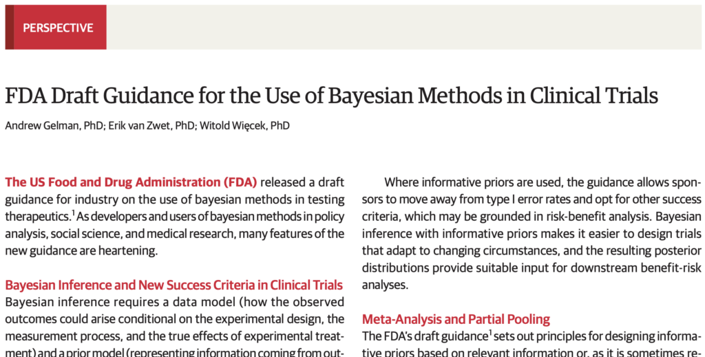
Some of our key points:

The prior is sometimes described as a subjective belief, but the FDA guidance frames it as pre-study information, which we think is a good framing. The formal and transparent incorporation of prior knowledge into the design and analysis of trials is the main advantage of the Bayesian approach. The use of prior information, even if not in a formal Bayesian framework, is not new in the context of clinical trials. For example, it is used during the planning stage of a trial using traditional frequentist methods to determine the sample size. . . .

The guidance still insists on type I error control when Bayesian methods are used, but only when the prior is noninformative. We see the logic to this: Bayesian analysis with noninformative priors is functionally similar to a traditional frequentist analysis, and in these cases there is no compelling reason to break with the current paradigm. In contrast, when substantial prior information is available, the required assumption for defining type I error of no treatment effect may already be inconsistent with that prior information to some extent, invalidating the type I error rate as a meaningful design metric. . . .

We suggest two simple rules for Bayesian analysis of clinical trials: (1) the prior should be clearly stated and (2) readers and reviewers should be able to assess the prior’s influence on the result. . . . The guidance is right to stress the importance of justifying the prior. However, we also remind readers that it is just as critical to have a prespecified and valid data model. Both the prior and the data model should be scrutinized when the data arrive, and it may be necessary to revise either. We also applaud the recommendation that computations be evaluated using simulation studies: in the Bayesian framework, these would be posterior predictive checks, in silico replicated datasets simulated from the fitted model that are then compared with the observed data, with systematic discrepancies indicating problems with the model. . . .

Although often criticized as subjective, Bayesian approaches, when implemented transparently, can improve on informal principles of clinical judgment that often inform the current FDA model.

Two other discussions

Along with our article, JAMA ran two other comments on the FDA guidance:

Embracing Bayesian Methods in Clinical Trials: FDA’s Long-Awaited Draft Guidance, by
Jack Lee, Frank Harrell, Lisa LaVange, and David Spiegelhalter.

Reflections on FDA Draft Guidance on Bayesian Methods in Trials—Protecting Scientific Integrity and Evidentiary Standards, by Scott Evans, Thomas Fleming, Holly Janes, and Lori Dodd.

Both groups of authors have lots of experience on the statistical analysis of clinical trials, and both articles are thoughtful. I recommend reading them both.

Comments on the pro-Bayesian discussion by Lee et al.

Lee at al. share our general perspective, and their comment is usefully complementary to ours. We focus on priors, hierarchical modeling, and meta-analysis, while they go into more detail on the way that Bayesian methods connect to classical methods and existing regulatory approaches.

I only have three nits to pick on their article. First, they refer to “skeptical, optimistic, or noninformative prior distributions.” I’d like to clarify that there are too sorts of “skeptical prior.” One version of a skeptical prior is centered at a negative value, i.e., you assume the prior model in which the effect is more likely to be negative than positive, so that to get a positive estimated effect you need strong positive information from the new trial. The other version is centered at zero, which corresponds to a world in which most effects are small (as in the priors on the signal-to-noise ratio discussed here). By default with clinical trials we recommend that second sort of skeptical prior.

Second, Lee et al. write, “By contrast [to classical p-values and confidence intervals], Bayes tackles the real question of interest head-on and provides a direct answer to the question ‘Does the new drug or biologic work?’ by computing the probability of treatment benefit.” I get what they’re saying, but I don’t like the binary framing of whether something works or not. Effects will vary by person, across situations, and over time; there’s not really a stable effect or average effect, and even if we’re summarizing by an average, the question is not whether this average is different from zero or even whether it’s positive, but how large it is. Sure, you can take your Bayesian inference distribution and summarize it by the posterior probability that the average treatment effect is positive, but that’s just one thing to look at, and I think it’s a mistake to identify this as “the real question of interest.”

Third, for reasons I’ve discussed many times, I’m not happy with their use of the term, “prior belief”–unless they’re also willing to refer to other aspects of statistical models as “belief.”

But these are all just minor issues of emphasis. In practice I expect that Lee et al. are recommending the same sorts of Bayesian methods for design and analysis of clinical trials as we are.

Comments on the Bayes-wary discussion by Evans et al.

The article by Evans et al. expresses much more skeptical about the use of Bayesian methods for clinical trials. As noted above, I find their article to be thoughtful and it is worth reading. But they do say some things I disagree with.

The good news is that I think that some of their concerns can be directly addressed, and I hope that after reading my comments they will revise their view somewhat.

You might say that Evans et al. have a strong prior against Bayesian methods, and in this comment I’m sharing information that should shift their prior a bit. As a Bayesian, I can hardly complain that they have strong priors, and it’s my duty to provide arguments that they will view as convincing evidence.

Evans et al. conveniently provide a list of key points:

I’ll go through their five points in turn.

Item 1: I agree 100%. “Replicability, integrity, and reliability of evidence for disease treatment and prevention.”

Item 2: Again, I agree completely in this list of settings where Bayesian methods have been useful.

Item 4: Again, I agree! Transparency about all aspects of design, data collection, and modeling is absolutely necessary. This is the case for non-Bayesian method and for Bayesian approaches as well. I also agree that Bayesian inferences based on informative priors should be accompanied by results with noninformative priors or non-Bayesian estimates. It’s important to see the effect of the prior.

Item 5: Again, complete agreement. FDA guidance is crucial.

So it all comes down to item 3.

Item 3: They write that Bayesian methods “can compromise evidentiary and integrity standards.” I agree: any statistical method can be used inappropriately, and we should be aware of failure modes, especially in a high-stakes situation such as clinical trials. They list three concerns: “concession of the benefits of randomization,” “loss of objectivity by incorporating sponsor- or investigator-specific priors,” and “reduced robustness via reliance on strong and sometimes unverifiable assumptions.” I think they’re just wrong on the first of these items. We discuss the issue more fully in Bayesian Data Analysis (see chapter 8 of the third edition), but, just quickly, Bayesian analysis of clinical trials makes strong use of the benefits of randomization, as this is what allows you to set up a likelihood function corresponding to an unbiased estimate. I don’t see any concession of the benefits of randomization, in design or analysis. For their second item, yeah, if you put in a bad prior you can get a bad posterior, and that’s one reason we emphasize transparency in any statistical analysis. See the last paragraph of our article above. Finally, yes, I agree that Bayesian inference has additional assumptions beyond a classical analysis. I don’t think this “compromises evidentiary standards,” though! The prior is based on evidence too.

Let me put it another way. Sometimes you’ll have a nice clean trial, no problems with recruitment, dropout, or missing data, precise and well-targeted measurements, and a large enough sample size to get precise inference for endpoints of interest. You can do a Bayesian analysis if you want, but it won’t make much difference, and the classical confidence interval should be just fine. In other settings, your data are noisy, there are various sources of bias, you’re interested in small subgroups, and classical inferences aren’t enough. You’re in the position of making decisions based on incomplete information. And here the Bayesian approach can be helpful. Yes, additional assumptions are required–I’d like to frame that as, “additional information can be added to the analysis”–; that’s the price you pay for adjusting for bias and noise.

All this explains why I agree with Evans et al. that it’s good to compare any Bayesian inference to the (potentially biased and noisy) classical estimate, and it’s important to be transparent about all assumptions–including the past data and theory used to construct the prior. Data models can be constructed badly (for example, adjusting for age or smoking using binary indicator variables, or using curves that don’t fit the data, or not accounting for hierarchical structure), and priors can be constructed badly too (for example, by centering your prior from a noisy past estimate). Transparency doesn’t eliminate these problems but it should help us notice and correct them when they happen.

Summary

General caution by skeptics of Bayesian methods is valid and should be applied more generally, to all of our statistical models.

A useful analogy is to regression adjustment for experiments and observational studies. If your experiment is clean and your noise level is low, you might be able to get away with a simple treatment vs. control comparison with no adjustment. But in real-world studies there are a lot of reasons to adjust for pre-treatment predictors–it can help even in the simplest experimental settings. That said, it’s good to compare adjusted to unadjusted results and to understand your adjustment procedures as they get more complicated.

The reason for Bayesian methods in clinical trials is that classical methods are often not enough. It’s good to see these new FDA guidelines, and I think JAMA got some good discussions that should help move the ball forward.

P.S. There’s this funny thing . . . the JAMA style required us all to write “bayesian” as lower case. I told them this was nonstandard but they insisted on it. Weird, huh?

P.P.S. More here from Frank Harrell.

Nutpie: state-of-the-art mass matrix adaptation for HMC

This post is from Bob

Nutpie laps NUTS

The short story is that the Nutpie sampler is usually twice as fast as Stan’s sampler for Stan models and twice as fast as PyMC’s samplers for PyMC models. The speed improvement is due entirely to better mass-matrix adaptation. Everything else is the same—dual averaging for step size adaptation and the biased-progressive, multinomial no-U-turn sampler for Hamiltonian Monte Carlo. Note that the speed is not coming from Python or Rust; we have a C++ implementation in the works we plan to interface with Python and then R.

The backstory

Adrian Seyboldt, a member of PyMC Labs, designed the sampler and released the open-source implementation linked above. He built it so he could try out Rust! Adrian’s also behind Stan’s game-changing new sum-to-zero parameterization along with Sean Pinkney. He’s a physicist by training and has amazing geometric intuition.

I tried Nutpie and it didn’t disappoint. So I wanted to understand the algorithm. I couldn’t understand the Rust code and Adrian hadn’t written any pseudocode or algorithm description. Eliot Carlson, with a recently minted MA in stats from Columbia, showed up at my office on the recommendation of Philip Greengard to look for a computational stats project. I asked him what he thought about Rust and like any great grad student, he wasn’t daunted by the fact that he knew nothing about Rust and was a statistician by training. With serious digging and some help from Adrian, Eliot extracted pseudocode descriptions and we were able to formulate the algorithm in what I hope is an understandable way. Eliot now works full time at PyMC Labs.

The paper

The arXiv paper just came out yesterday.

We’d love to hear any comments, corrections, or suggestions people might have.

My role in this was just helping to formulate the whole thing as a stats paper in a language that computational statisticians could understand. Adrian and Eliot worked out the proofs, from which I learned a lot.

Why is Nutpie better?

There are two basic reasons why Nutpie’s diagonal mass-matrix adaptation is better than Stan’s:

1. Better initialization: Use the gradients at the initial point to estimate mass matrix and make the whole sampler scale invariant.

2. Two sources of information: Use the position and the gradient of the log density at the position as two sources of information with which to estimate a mass matrix

The motivation for (1) is that the outer product of the scores is a one-sample Monte Carlo estimate of the expected negative Hessian of the target log density. The one-sample estimate is regularized by taking a geometric average with an identity matrix—using a few more draws here may be more stable.

Will wonders never cease, but it turns out to be relatively simple to take the geometric mean as the midpoint of a geodesic in the affine-invariant Riemannian manifold (AIRM) of positive-definite matrices. It works out to regular geometric mean in the diagonal case, making it simple to implement.

The motivation for (2) is that in a multivariate normal distribution with covariance Sigma, the covariance of the draws is Sigma and the covariance of the scores (gradients of log density of the draws) is Sigma inverse. These are then geometrically averaged to produce an estimate. This can converge very fast—many fewer iterations than the dimensionality of the problem.

As with Stan, the default in Nutpie is to use a diagonal mass matrix. Unlike Stan, Nutpie also lets you use a low-rank plus diagonal approximation (as in L-BFGS optimization), which can go a long way to decorrelating hierarchical models. Using a rank K approximation, what would otherwise be N^3 operations like solves or matrix products become K^2 * N, which is manageable for K of order 10 or less.

Mathematical motivation

The geometric average of the covariance of the draws and the inverse covariance of the scores minimizes the Fisher divergence from a standard normal distribution to the preconditioned target density. Fisher divergence is like Kullback-Leibler divergence, but instead measures the expected distance between gradients rather than the difference between log densities. This turns out in practice to lead to a better diagonal preconditioner. The paper provides proofs and an appendix with geometric motivations.

What we do not prove and what I do not believe anyone understands is how to select an optimal static preconditioner when the target log density has varying curvature, in any form: diagonal, low rank plus diagonal, or dense. I think what we really need is dynamic adaptation that isn’t cubic like Riemannian and doesn’t require implicit integrators.

A data model is not just a “likelihood”

This blog post is by Aki with some excerpts in the end from the forthcoming Bayesian Workflow book Section 5.4 A data model is not just a “likelihood”.

It seems to be increasingly common that people say likelihood when they talk about the data model.

A Bayesian model is defined by the joint distribution of the data and parameters p(y, theta). This is usually factorized as data model p(y | theta) and prior p(theta). The product of data model and prior defines the joint distribution.

When we condition on data, p(y, theta) is only a function of theta and Bayes’ rule gives the posterior as p(theta | y) propto p(y | theta) p(theta). Here p(y | theta) as a function of theta is called likelihood (function).

I have intentionally used the common notation where p(y | theta) as a function of y is the data model and p(y | theta) as a function of theta is likelihood (function). Due to this common notation, it is even more important that we use the correct names for these.

For example, with a Bernoulli data model, the data model is discrete but the likelihood is continuous. Clearly they are completely different functions. A very long time ago, a student asked “How is it possible that combining a discrete binomial model and a continuous beta prior gives a continuous posterior?”. So it is crucial to understand that the likelihood function is not binomial but has the shape of a beta function!

We need generative models, data models, for prior checking. If you combine the likelihood and prior you get the posterior. If you combine the prior and data model, you get the prior predictive distribution!

You can’t always figure out the data model from the likelihood. The classic example is a (discrete) Poisson model for the number of events in a given time and a gamma model for the waiting time until a certain number of events. Both have gamma-shaped likelihoods, and knowing that function does not tell us what the data model is!

When, for example, in Stan you write

y ~ normal(mu, sigma);

this is read “y is distributed as normal with parameters mu and sigma”.

We can also write

target += normal_lpdf(y | mu, sigma);

and if y is data, then we are incrementing target with log-likelihood.

In simple models, the data model is easy to distinguish from the prior. But with hierarchical and missing data models there is no sharp division between parameters and data, as a model can have latent data that are not observed but are still given a generative model. For example, in the case of partially censored data, we may have observations y_obs and censored observations y_cens for which we know that they are larger than a known censoring threshold 𝑈. We can write a joint model (as this blog doesn’t allow equations, here’s a screenshot from the Bayesian Workflow book)

Here, y_cens are given the same generative data model as y_obs, and U doesn’t have a model at all. If we define the model before the data are observed, then it is not possible to say in a model like this where the data model ends and the prior begins. It depends upon which observations are censored, once the data arrive.

Another screenshot from the Bayesian Workflow book:


And yet another example:


I hope these examples illustrate why it is important to correctly use the terms data model and likelihood, and not call everything likelihood. In easy cases it is possible to understand from the context when the term likelihood is wrongly used, but if you keep using it in simple cases, you make things difficult in more elaborate cases.

We discuss data models and likelihoods much more in the forthcoming Bayesian Workflow book (expected publication date in June).

ps. A data model is also sometimes called the sampling distribution, the observation distribution, or the residual distribution; these correspond to different data structures (sampling from a population, noisy measurement of a latent process, and residuals from an additive model). We use the more general term “data model” to allow for all these scenarios.