7 1/2 Schools—mistakes were made

Mitzi Morris sends along the paper trail (I love archaic idioms) for her data spelunking in advance of her all-day introductory Stan tutorial next week at StanCon (we’ll see you in Uppsala). She was trying to reproduce the results from my decade-old case study on hierarchical modeling when she ran into a couple discrepancies.

The case study was designed to provide a Bayesian replication of the results in Efron and Morris’s five decade old paper on hierarchical modeling (aka Stein’s estimator, aka population regularization, aka “empirical” Bayes), which is still under a paywall courtesy of our “friends” at the American Statistical Association. If your organization isn’t paying ASA for access to a paper that an academic donated for free 50 years ago, I’ll leave you to find your own pirated copy in good conscience, or you can follow the link and let Google hoist the Jolly Roger for you (now that’s an even more obscure and archaic reference).

My case study’s been out for ten years. Mitzi found a problem when matching the data provided in the R package pscl against that in Efron and Morris’s paper. In particular, the data for the player named “Williams” was wrong. Efron and Morris manually transcribed the data from a newspaper with the goal of finding a bunch of players with the exact same number of at bats on a given day (45, it turns out). They did so accurately.

Sadly, I imported an error in the 18-item data set from the R package. Here’s an edited report from Claude after it tracked down what went wrong.

  1. The 1975 paper is correct, although it only gives the surname “Williams.”

  2. The R package pscl expanded that name incorrectly to Billy Williams, while retaining Walt’s team and remaining-season data. Published pscl data.

  3. The Bean Machine tutorial () contains the exact mixed row found in your CSV:
      Billy,Williams,...,591,0.3299,636,205,0.251
    

  4. That row combines Billy Williams’s at-bats and hits with Walt Williams’s .251 average. Thus, ID 15 in your data should be corrected throughout to:
      Walt,Williams,45,10,0.222,270,0.2556,315,79,0.251
    

But wait, that’s not all. There was another typo in the Bean Machine tutorial. They mistranscibed Ron Swoboda‘s surname as “Swaboda.” I should have caught that as I was a huge baseball fan in the early 1970s, am an excellent speller, and grew up around a lot of Poles and Czechs in Detroit and its western suburbs. Mitzi then had the following conversation with Claude after she noticed the typo. This may be the first time I’ve seen Claude crack a spontaneous joke.

Mitzi: did that [the typo] come also from the R file?

Claude: If you mean the Swaboda misspelling: no. The pscl R dataset correctly uses Ron Swoboda. The misspelling appears in the Bean Machine tutorial
(https://beanmachine.org/docs/overview/tutorials/Hierarchical_modeling/HierarchicalModeling/), which contains Ron,Swaboda.

Mitzi: are you sure? I’ve heard it both ways.

Claude: Yes—despite what Shawn Spencer might say, it is definitively Ron Swoboda, with an o.

Mitzi: who’s Shawn Spencer? in 2017, Bob Carpenter published this dataset in a Stan case study.

Claude: Shawn Spencer is the fictional detective in the TV comedy Psych, played by James Roday Rodriguez. “I’ve heard it both ways” is his recurring response when someone corrects him—hence my reference.

Mitzi and I use “I’ve heard it both ways” all the time, having watched umpteen seasons of Psych. I would recommend if you want a lighthearted detective story that doesn’t take itself too seriously with lovable characters and you can put up with the ubiquitous mid-00s background sexism and racism.

Walnutpie version 0.0.1 Released

We are happy to announce the official release of Walnutpie version 0.0.1.

Walnutpie is an MCMC sampler for continuously differentiable densities coded in Python, accepting models coded in Stan, PyMC, NumPyro, JAX, and plain old Python.

Walnutpie is not an official Stan project

I thought this was worth saying up front. It may eventually migrate to Stan, but for now, we followed the Nutpie approach of building a standalone sampling package that worked with a range of packages for defining models.

R version

We plan to develop an R interface after we release version 1.0.0 of the Python interface. So hopefully in 2026.

pip installable

Walnutpie is on PyPI, so it’s pip installable. The documentation includes information on getting started, running models, and posterior analysis. We have not yet included case studies for modeling tools other than Stan and Python.

Stan through C++

Walnutpie runs Stan models through C++ using BridgeStan, so there is no Python dispatch overhead for Stan sampling. The basic architecture of the API is based on Adrian Seyboldt’s sampler Nutpie. We are working on doing that for other packages like NumPy and JAX to the extent that we can.

GitHub source

Development discussions and source code are managed through GitHub.

Features of Walnutpie

We are almost ready to release the paper on arXiv with all of the gory pseudocode details of all of the algorithms used for Walnutpie. It will explain the following points in detail.

  1. Walnuts: The underlying Hamiltonian Monte Carlo sampler is Walnuts. Walnuts uses Nuts for choosing the number of steps per iteration. It further allows step sizes within the Hamiltonian dynamics simulation to be lowered when necessary to preserve simulation accuracy. This helps with robustness and with accuracy in multi-scale distributions (i.e., ones where the curvature as represented by the Hessian varies around the posterior). With a high tolerance threshold, Walnuts reverts to Nuts’s behavior.

  2. Mass-matrix warmup: The mass-matrix warmup strategy is an online form of Nutpie (links to: the paper and software). Nutpie minimizes Fisher divergence by estimating the inverse mass matrix as the midpoint (in the appropriate manifold) between an estimate based on the variance of the draws and the covariance of the scores (gradients of the log density). The target is better than Nuts’s variance of draws in both convergence speed and sampling efficiency. Walnutpie only supports diagonal mass matrices (Nuts supports dense matrices and Nutpie supports low-rank plus diagonal and even more general normalizing flow approaches). The approach is online in the sense that it is not blocked like warmup in Nuts or Nutpie—it updates every iteration by exponentially discounting the past to mimic Stan’s exponentially increasing history sizes. We also borrow Nutpie’s mass matrix initialization based on a regularized outer product of gradients at the initial point.

  3. Step-size warmup: The step size adaptation strategy has not changed, but the underlying stochastic gradient descent algorithm is Adam rather than dual averaging. We found Adam to be faster to converge and much more stable. Matt Hoffman included a hack in the original Nuts approach to stabilize dual averaging, but even with that it is not as stable as Adam.

  4. Concurrency and automatic stopping: The underlying sampler is multi-threaded (using C++11 threads) with shared data. On top of the multi-threading, we have layered a convergence monitor in a separate thread that communicates with the chains through lock-free, latest-only, single-producer/single-consumer (SPSC) buffers (specifically, a triple buffer). The monitor automatically stops warmup when the mass matrices and step sizes have converged within tolerance to their cross-chain averages. The monitor automatically stops sampling when a target (traditional, non-split, non-ranked) R-hat; threshold is satisfied for the unnormalized log density, which typically converges more slowly than any of the individual parameters. It can also be configured to run for a fixed number of warmup and/or sampling iterations. The link between the original R-hat and effective sample size makes this essentially an unscaled ESS target.

  5. Ragged chain summaries: Asynchronous concurrent execution of chains with automatic stopping produces chains of different lengths. Because ArviZ does not accept ragged chain input of this kind, we have included posterior analysis tools for means, variances/standard deviations, quantiles, traditional R-hat, effective sample size, and Monte Carlo standard error that work with ragged chains.

  6. C++20: Walnutpie is implemented in C++20. As a programming language type fanatic (I’ve written two books with “type” in the title!), I don’t know how I survived without C++ concepts before C++20.

  7. ctypes FFI: The foreign function interface in Python uses ctypes rather than a higher-level interface, which sidesteps the requirement of ABI compatibility of C++ binaries.

Developers

We would also like to welcome new developers who may want to get involved. There are already a stack of improvements we’d like to make, which we have enumerated on the GitHub issues.

Sources of algorithms

The Walnuts algorithm was a joint effort among Nawaf Bou-Rabee, Sifan Liu, Tore Kleppe, and Milo Marsden. Nutpie was developed by Adrian Seyboldt. Nuts, in the form used currently in Stan, was originally developed by Matt Hoffman and Andrew Gelman, then improved with multinomial sampling and mass matrix adaptation by Michael Betancourt. We haven’t yet added cross-chain adaptation as developed by Ben Bales, but the pieces are all in place to do so.

Brian Ward and I wrote all of the version 0.0.1 code with design advice and code review from Steve Bronder. Claude (the LLM) helped with code review and testing, but we didn’t use it to write the actual code (not out of principle, but because Brian and I both prefer the control of doing things manually).

Feedback

We would very much appreciate any feedback people have, including feedback on the documentation and ease of use, the source code, and performance.

We are happy to get feedback through issues on GitHub, through replies to this post, or through mail to one of the developers.

Bayesian Workflow exists as a physical book!

We’re very excited about this book. It’s the result of several years of effort. You can order from the publisher or from Amazon.

Here’s the book’s webpage, which includes the data and code for the book’s examples and case studies, of which there are many.

Here’s the table of contents:

Part 1: From Bayesian inference to Bayesian workflow
1. Bayesian theory and Bayesian practice
2. Statistical modeling and workflow
3. Computational tools
4. Introduction to workflow: Modeling performance on a multiple choice exam

Part 2: Statistical workflow
5. Building statistical models
6. Using simulations to capture uncertainty
7. Prediction, generalization, and causal inference
8. Visualizing and checking fitted models
9. Comparing and improving models
10. Statistical inference and scientific inference

Part 3: Computational workflow
11. Fitting statistical models
12. Diagnosing and fixing problems with fitting
13. Approximate algorithms and approximate models
14. Simulation-based calibration checking
15. Statistical modeling as software development

Part 4. Case studies
16. Coding a series of models: Simulated data of movie ratings
17. Prior specification for regression models: Reanalysis of a sleep study
18. Predictive model checking and comparison: Clinical trial
19. Building up to a hierarchical model: Coronavirus testing
20. Using a fitted model for decision analysis: Classification competition
21. Posterior predictive checking: Stochastic learning in dogs
22. Incremental development and testing: Black cat adoptions
23. Debugging a model: World Cup football
24. Leave-one-out cross validation model checking and comparison: Roaches
25. Model building and expansion: Golf putting
26. Model building with latent variables: Markov models for animal movement
27. Model building: Time-series decomposition for birthdays
28. Models for regression coefficients and variable selection: Student grades
29. Sampling problems with latent variables: No vehicles in the park
30. Challenge of multimodality: Differential equation for planetary motion
31. Simulation-based calibration checking in model development workflow

Appendices
A. Statistical and computational workflow for Bayesians and non-Bayesians
B. How to get the most out of Bayesian Data Analysis

One way to think of the book is that it’s all the things missing from BDA, like how to set up an informative prior, what to do when your computations aren’t converging, how to work through a series of models fit to the same data, how to design and perform simulated-data experiments . . . and all sorts of other things too.

The core of the book–parts 1 through 3–clock in under 200 pages, and then we have another 300 pages full of case studies demonstrating different aspects of Bayesian statistical and computational workflow. The appendices should be useful to you too, first because the workflow ideas in this book apply to non-Bayesian inference too, and second because BDA still has lots of valuable material in it, so it’s good to know where to look.

This new Bayesian Workflow book could change your life (we hope), and I thank my coauthors, Aki Vehtari and Richard McElreath, with Daniel Simpson, Charles C. Margossian, Yuling Yao, Lauren Kennedy, Jonah Gabry, Paul-Christian Bürkner, Martin Modrák, Vianey Leos Barajas, for all their care and effort. We thank our employers and various funding agencies for giving us the resources to be able to write this book as a side project along with all our daily responsibilities. And we thank many people for their input on earlier versions of the book, along with the Stan developers making so much of this work possible and the Stan community of users for supplying a continuing series of challenges that have motivated many of the ideas and methods discussed in the book.

I posted this already on the blog and you can see answers to some questions in the comments there. I’m posting it again here because, hey, we don’t come out with a new book every day!

I hope you find the book readable, interesting, and useful.

Structural equation modeling (SEM) and positive definiteness

This post is from Bob.

Mitzi and I were swotting up on structural equation models (SEM) for our class this past Monday at the Modern Modeling and Methods (M3) conference at Fordham University. It was a lot of fun and now I think I understand SEM notation. I really like these applied conferences and this was a group of psychometrician, econometricians, and sociometricians. Many if not most of them thought about models in terms of SEM, so we thought we should figure it out. But I was left with a concern you may be able to help me sort out.

The example

The first worked example in Ken Bollen’s seminal 1979 textbook on SEM is a study of how industrialization relates to democracy. It comes from his paper,

  • Bollen, Kenneth A. (1979). “Political Democracy and the Timing of Development.” American Sociological Review, 44(4).

and was reprised in his book

  • Bollen, Kenneth A. (1989). Structural Equations with Latent Variables. Wiley.

I had the pleasure of sitting across from Ken at the invited speakers dinner at the conference, so I’m glad I looked into SEM before that. Good news for the SEM devotees—he released a completely revised guide to SEM a few months ago.

The data and parameters

The data consists of eleven covariates (called “indicators” in SEM) for each of 75 countries. Four of the covariates are related to democracy in 1960 (y1, y2, y3, y4), the same four measurements were taken again again in 1965 (y5, y6, y7, y8) , and there were three measurements of industrialization in 1960 (x1, x2, x3).

The SEM model the original researcher came up with here assumes three latent scalars per country, industrialization in 1960 (IND60), level of democracy in 1960 (DEM60), and level of democracy in 1965 (DEM65). These latent parameters are related in the following way: democracy in 1960 is a regression on industrialization in 1960, and democracy in 1965 is a regression on both democracy in 1960 and industrialization in 1960.

The covariates are then modeled like a seemingly unrelated regression in econometrics. The four democracy 1965 parameters are treated as regressions on the latent level of democracy in 1965, and similarly for the democracy in 1960, and industrialization in 1960.

Rather than independent errors, a SEM model explicitly indicates with arrows which pairs of observations are allowed to have non-zero correlation in the covariance matrix for the observations. The three industrialization observations are assumed to have zero correlation—there are no arrows between any of the three measurements in the SEM diagram. Each of the four measurements in 1960 is assumed to covary with the same measurement taken in 1965. In addition, the second and fourth measurement in each year are assumed to be correlated with each other, which leads to a box-like structure.

The SEM diagram

Here are the arrows in the diagram, where I’m not using their standard LISREL notation, but writing them in R expression syntax to indicate what is regressed on what. In their graphical notation, just replace ~ with <-. All three latent variables and all eleven measurements are indexed by country.

IND60
DEM60 ~ IND60
DEM65 ~ DEM60, IND60

x1, x2, x3 ~ IND60
y1, y2, y3, y4 ~ DEM60
y5, y6, y7, y8 ~ DEM65

The covariance structure is indicated by stating which pairs of measurements are modeled with non-zero correlation. The first four just pair the measurements of the same thing across 1960 and 1965.

y1 <-> y5
y2 <-> y6
y3 <-> y7
y4 <-> y8

The last pair of correlations are within 1960 and within 1965.

y2 <-> y4
y6 <-> y8

Together, these induce an odd box structure, where y2 is correlated with y6 and y4, both of which are correlated with y8, but y2 and y8 are assumed to have zero correlation.

y2 <-> y6
^      ^
|      |
v      v
y4 <-> y8

Stan implementation

We didn’t get this far in my half of the class, so I will share here the Stan Playground example where I fit Bollen’s example (you can get the data and the Stan model through the Playground link:

It gets the right answer compared to lavaan/blavaan, which is nice. In the Stan code, xi is IND60 and eta1, eta2 are DEM60, DEM65. The relation among the latent parameters are modeled directly as regressions. The correlations among the observations are modeled using soft zeroing, where I just put a tight prior around zero on the structural zero elements, because Stan doesn’t give you a good way of setting up structural zeroes in a covariance matrix (Sean Pinkney or Ben Goodrich might know how to do this?).

This makes me curious how the lavaan package in R manages this. There’s a Bayesian version of lavaan built on top of Stan, blavaan. The first example right at the top of the home pages for both the lavaan and blavaan is Bollen’s democracy model. I guess it’s like the Scottish lip cancer data set for spatial modeling or Fisher’s iris data for regressions.

My questions

Consider a simple diagram among measurements like the following.

x <-> y
y <-> z

This says there can be non-zero correlation between A/B and also between B/C, but the correlation between A/C is zero. It’s a simplified case of the box we saw in the actual example. These arrows implies the correlation matrix looks as follows.

|        1  rho[x,y]         0 |
| rho[x,y]         1  rho[y,z] | = Omega
|        0  rho[y,z]         1 |

Given that the correlation matrix Omega must be positive definite, this limits the range of rho[x,y] and rho[y,z]. For example, we can’t have rho[x,y] = rho[y,z] = 0.9, or rho[x,z] would have to be greater than zero to maintain positive definiteness.

Q1: Why doesn’t SEM instead say that the correlation rho[x,z] is just the minimum value it can be given rho[x,y] and rho[y,z]? I’m suggesting that we instead treat the above diagram as implying no additional correlation between x and z other than that implied by the correlation between x and y and the correlation between y and z? That is, why try to shrink rho[x,z] all the way to zero? From the text, it feels like the motivation is to enforce zero correlation in the model. But all this is doing is simplifying regressions—it won’t actually enforce zero correlation among the measurements that are modeled with zero correlation. I wished I’d asked Ken this question at dinner, but I’ll ping him about this blog post and hopefully get a response.

Of course, in the pragmatic Bayesian workflow, we’d use posterior predictive checks to evaluate whether there’s unmodeled correlation between x and z.

Q2: I’m also curious what Andrew and others think about enforcing structural zeroes in correlation between measurements as opposed to just estimating a dense covariance matrix and inspecting where the correlations fall.

LLM-generated Stan case study on Galileo’s inclined plane experiment

This post is from Bob.

I’ve been planning for at least a couple years to generate a case study around Galielo’s use of an inclined plane instrumented with water clocks to estimate the terrestrial gravitational constant. Here are some photographs of a replica in the Museo Galileo (click to blow them up). And here’s a video simulation of the experiment. We replace his clever pendulum apparatus explained in the video and the web page with simple Bayesian statistics so we can actually estimate the gravitational constant.

The case study

Here is a draft.

Bob Carpenter. 2026. Estimating g from Galileo’s Water Clock: A scientific Bayesian inverse problem with Stan and CmdStanPy. GitHub.

I list myself as the author here because I’m responsible and AIs can’t own copyright in the U.S., but 100% of the text and code was written by Claude Opus 4.8 (medium or high effort, but I can’t recall which). I used the desktop app, which doesn’t allow sharing, but you can try it yourself.

The prompt

Here’s the sloppy prompt I used, which I just typed in without much thought in a couple minutes to get a feel for what it could do on its own.

I would like to generate a case study written in Quarto and using CmdStanPy to demonstrate solving scientific Bayesian inverse problems. I want to use a simulation of Galileo’s water clock experiment, which can be used to estimate the gravitational constant. I would like you to start by generating the mathematical model description in LaTeX, the model code in Stan to solve the inverse problem, and a simulation driver in Python using CmdStanPy and plotnine for plotting. Please just `import plotnine as pn` and use `pn.geom…`, etc. All I need in the output now is a call to `.summary()` on the fit returned by `.sample()`. Wrap this all up in a quarto document for me from which I can generate HTML by calling `quarto render galileo.qmd`.

It was done before I got back to my desk with a cup of coffee (well under five minutes). So not quite the several hours Andrew said it took him to write his case study on the New York Knicks basketball team, which he posted earlier today. Of course, this was much simpler and I didn’t have to think through any details before generating it.

Is it right?

What Claude produced looks really good to me. If a student had done this, I’d given them an A. I can’t object to the way it described Galileo’s experiment, wrote the math, wrote the Stan code, wrote the Python simulation, or plotted the raw data as Andrew is always urging us to do.*

The source

You can find the source .qmd file on my GitHub:

https://github.com/bob-carpenter/case-studies/tree/master/galileo-gravity

It’s short, so I would have just included it, but the blog software blocked my post after considering it an attack on the site. To get it to render with resources embedded, I had to ask Claude a follow-up question and manually insert a single line of config into the .yaml header for the markdown document.

Putting this blog post together took longer than writing the prompt and checking the results.


*   Maybe Claude runs a little simulation of Andrew like I do. Andrew himself claims to run a simulation of Jennifer Hill—it’s the basis of his
handy statistical lexicon entry for “WWJD,” which he told me stands for “What would Jennifer do?” Unfortunately, neither the lexicon entry nor its underlying link explains the acronym.

Call for invited session proposals for the upcoming BayesComp conference

Lu Zhang writes:

As a member of the BayesComp 2027 conference committee, I would like to share the announcement of the call for invited session proposals for the upcoming BayesComp conference, which will be held in College Station, Texas, on May 18–20, 2027.

The scientific committee is currently soliciting proposals for invited sessions. Each invited session will consist of three speakers, and proposals should focus on timely, important, and broadly engaging topics in Bayesian computation and related areas.

The submission deadline (as of now) for invited session proposals is August 15, 2026.

Proposal form: https://forms.gle/wpYvkkjKGZ5vHqhF6

Additional details are available in the official announcement:

The LOC for BayesComp 2027 is pleased to announce that the next edition of BayesComp will take place in College Station, TX during May 18–20, 2027. The scientific committee is now opening calls for invited sessions. Each invited session will consist of 3 speakers. Proposals should highlight timely, important, and broadly engaging topics in Bayesian computation and related areas. Each speaker may be listed as a speaker in only one invited or contributed session proposal.

Lu is the first author on the Pathfinder paper and continues to do interesting work on Bayesian statistics and computing. Based on what I’ve heard about past BayesComps, the conference should be really interesting.

Full day Stan tutorial at Modern Modeling Methods (M3) this summer in New York (22 June 2026)

This post is from Bob

Mitzi Morris and Bob Carpenter, two of Stan’s developers, will be presenting a tutorial on Stan and Bayesian data analysis aimed at psychometricians this summer.

Abstract

This workshop is a full day, hands-on introduction to Bayesian modeling and statistical inference using the probabilistic programming language Stan.

The course will be organized around the key properties of Bayesian statistical modeling for science, including the nature of uncertainty, modeling a generative process through a data generating distribution, modeling existing knowledge through a prior, and pushing uncertainty through inference. As we do this, we will show how Stan can be used to both code the models and perform statistical inference for quantities of interest, be they retrospective parameter estimates or prospective predictions or forecasts. We will concentrate on full Bayesian posterior inference, including a discussion of calibration, model checking for both prior and posterior inference, and model comparison with cross-validation. We will spend some time showing how some structural equation models (SEM) can be translated directly to Stan and will also introduce psychological models for educational testing, crowdsourcing, rating and ranking, and real-time decision processes.

This class will require a notebook computer with a network connection (Wifi will be available in the classroom). We will use the Stan Playground, which runs Stan in the browser, which we will pre-populate with models of interest. We will probably also break into R or Python at various points to demonstrate methods not yet supported by the Playground, such as the brms regression expression language.

Andrew on psychometrics

Andrew once told me that any model you could come up with was probably invented by a psychometrician 50 years ago (make that 60—he said it at least 10 years ago). I have evidence that he’s right form the project that drew me into Bayesian statistics—crowdsourcing. Andrew and Jennifer Hill helped me formulate a crowdsourcing model where raters give you noisy measurements of underlying categorical variables (e.g., they answer survey questions about whether a word in context is a noun, for example, to use something I was working on at the time). Turns out Phil Dawid and A.P. Skene published the same model in 1979 in one of the earlier applications of the expectation maximization (EM) algorithm and they used natural language data (drawn from medical records).

The rest of the conference

The rest of the program looks really great—it’s just the kind of applied wrestling with real data that I like.

Speaking of Jennifer Hill, she’s one of the keynote speakers at M3. Every talk of Jennifer’s I’ve attended has been great. You may know her as Andrew’s co-author on the regression books, which I cannot recommend highly enough if you’re interested in this kind of applied modeling.

Beyond the conference

You see the same kind of Bayesian modeling focus for real data at venues such as ISEC (international ecology conference to which I went to once just because I like these models and these kinds of conferences), StanCon (see you in Uppsala in August!), and GeoMed (which Mitzi attends). I’m sure there are more in other fields. I’m always disappointed that there’s almost nothing like these kinds of nitty-gritty applied papers at ISBA (Nagoya this summer) or BayesComp (somewhere next year). The conferences about Bayesian statistics or computing that I’ve been to have all been super theoretical.

Jonah’s seminar tomorrow: “Bayesian Workflow and the Software That Shapes It”

This is Leo. Jonah Gabry (Stan developer, Andrew’s collaborator, etc.) is spending the whole month of May as a visiting professor here with us at the University of Trieste in Italy. Tomorrow, May 19th, in the De Finetti room at the University of Trieste, at  9 am NYC time (GMT-4), Jonah will give the following talk:

“Bayesian Workflow and the Software That Shapes It”

based on the upcoming book:  “Bayesian Workflow”.

For anyone local, you are welcome to come in person. Anyone else can join on Microsoft Teams (available here).

Alchemize: PyMC’s model to replace Stan/PyMC, etc. with an LLM

This post is from Bob

I’ll let Thomas Wiecki, who is one of the core PyMC devs and one of the partners at PyMC Labs, speak for himself here:

If you haven’t seen what people are doing with agentic AI, this is a good example. I’m really happy that Thomas and PyMC Labs are sharing their thoughts and initial tries at things like this as I think it has the potential to benefit everyone working on modeling.

If you want to see the basis of the agent’s instructions, check out the “skill” for PyMC that Chris Fonnesbeck wrote.

We’ve already batted this around a bit in email with Thomas, so I can summarize some talking points:

LLM-based chatbots are really good at translating. Compiling (or more technically correct, transpiling) a statistical model down to a language like Rust or C++ or JAX is a kind of translation.

You can start from PyMC’s execution trace, but you can also start with a model description. You could also start with something like Stan code.

The biggest bottleneck to deploying Bayesian models in my opinion is the inherent variance and unreliability of MCMC-based inference. Our workflow proposals are all about making sure this doesn’t go wrong. Wiecki’s point here is that we can have the bots go through the workflow. Iterating until the gradients and log densities match is a good example, but this could be extended to more parts of workflow.

The skills feel a lot like writing a textbook for a bot. I have no idea how hard or easy this is or how much it improves over the baseline. Jeremy Magland built a RAG-like helper for Stan that compressed the Stan Reference Manual down to 1K tokens for context (like a skill) and allowed it to search and import from the Stan User’s Guide, but never measured how much it improved over the baseline. It really feels like it should also have the Stan Functions Reference, BDA3, Regression and Other Stories, and the Bayesian Workflow book, as well.

Hopefully we’ll asymptote at writing a textbook sized set of skills and not have to write one per target model (that is, something like the Stan User’s Guide, Reference Manual, Functions Reference).

I’m curious as to whether it will eventually be able to make writing hard models easier. I’m thinking of efforts like epinow2, which involves a very large chunk of Stan code.

As the foundation models and chatbot tuning changes, there’s going to be an issue of regression testing and tuning for whatever the latest models are.

P.S. This effort explains how Thomas was able to create the huge posteriordb pull requests for PyMC (#320 and #319)!

P.P.S. The latest thing Claude (Opus 4.7) did that impressed me was generate the ess(MatrixXd, vector) function in summary.hpp. This function estimates effective sample size Stan style (discounting for R-hat > 1) on a ragged array of Markov chains. We have to generalize all the posterior analysis tools to deal with the new asynchronous parallel sampler). I had Stan’s ESS function and all the other functions I’d written for the ragged structures to give it as a guide. It’s very easy to code review that it matches Stan’s implementation for the new data structure. I only had to tweak the output a little bit for style.

Expanding the Stan User’s Guide

This post is from Bob.

The Stan User’s Guide has been evolving organically along with the project. I’m writing this post for two reasons—to let you know what we’ve added lately and to encourage you to add your own chapters.

History

Initialy there was just one doc that included what is now the Reference Manual, Function sReference and CmdStan Manual. You can browse them all on the web or download pdfs from the Stan documentation web site.

Most of the topics grew up opportunistically from either things the team was interested in, new features we added to Stan, or just trying to cover the basics of the chapters of Bayesian Data Analysis and Data Analysis Using Regression and Multilevel/Hierarchical Models.

Recent additions

There have been some recent additions, including some from new faces:

There are also a metric ton of minor clarifications, fixes, and model examples, such as Mitzi Morris’s additional sufficient statistics optimizations and you can simply look at all the documentation pull requests.

The future is you

You can see from Franziska’s pull request, Abner’s PR, and Brynjólfur’s PR that we provide a lot of guidance and feedback. I found it super useful to write a lot of the documentation when I was learning statistics because I got feedback from Andrew Gelman, Ben Goodrich, Aki Vehtari, and Michael Betancourt, among others.

Some topics that would be nice to add

There is a lot to add to our existing discussions and you can see a lot of that in the pull request list on our documentation repository. There are also many topics that we don’t cover or don’t cover well. Off the top of my head, roughly ordered near the top according to my assessment of how impactful it would be to add.

  • causal inference using Rubin’s potential outcomes framework
  • Thompson sampling for reinforcement learning/bandits (sorry, Andrew!)
  • penalized complexity priors and the Besag-York-Molie II spatial model (working from Mitzi’s Morris’s case study)
  • Extreme value models
  • RNA-seq and DNA-seq composition models at the read level and k-mer level
  • Econometric models (I don’t even know what these are, but there are books)
  • Stationarity-constraining parameterizations of VAR models a la Sarah Heaps
  • Neural networks
  • A/B testing (ideally sequential)
  • spatio-temporal models along the lines of Leon Held’s survey
  • non-trivial examples of ODE models like Lotka-Volterra (my case study), SEIR (Elizaveta Semenova et al.’s case study) or even better, pharmacokinetic/pharmacodynamic (multiple case studies around Torsten), soil carbon (my very early case study, but there’s been much better work since)
  • Hilbert-space approximations to Gaussian processes (GPs)
  • PDE approximations to GPs
  • Fourier space analyses of GPs
  • N-gram language models
  • Plackett-Luce model for contest with more than two players (this can follow my case study for StanCon)

Some of those may already be mentioned in our doc, so sorry if you’ve already written something. Also, feel free to suggest more topics in the comments.

Nutpie: state-of-the-art mass matrix adaptation for HMC

This post is from Bob

Nutpie laps NUTS

The short story is that the Nutpie sampler is usually twice as fast as Stan’s sampler for Stan models and twice as fast as PyMC’s samplers for PyMC models. The speed improvement is due entirely to better mass-matrix adaptation. Everything else is the same—dual averaging for step size adaptation and the biased-progressive, multinomial no-U-turn sampler for Hamiltonian Monte Carlo. Note that the speed is not coming from Python or Rust; we have a C++ implementation in the works we plan to interface with Python and then R.

The backstory

Adrian Seyboldt, a member of PyMC Labs, designed the sampler and released the open-source implementation linked above. He built it so he could try out Rust! Adrian’s also behind Stan’s game-changing new sum-to-zero parameterization along with Sean Pinkney. He’s a physicist by training and has amazing geometric intuition.

I tried Nutpie and it didn’t disappoint. So I wanted to understand the algorithm. I couldn’t understand the Rust code and Adrian hadn’t written any pseudocode or algorithm description. Eliot Carlson, with a recently minted MA in stats from Columbia, showed up at my office on the recommendation of Philip Greengard to look for a computational stats project. I asked him what he thought about Rust and like any great grad student, he wasn’t daunted by the fact that he knew nothing about Rust and was a statistician by training. With serious digging and some help from Adrian, Eliot extracted pseudocode descriptions and we were able to formulate the algorithm in what I hope is an understandable way. Eliot now works full time at PyMC Labs.

The paper

The arXiv paper just came out yesterday.

We’d love to hear any comments, corrections, or suggestions people might have.

My role in this was just helping to formulate the whole thing as a stats paper in a language that computational statisticians could understand. Adrian and Eliot worked out the proofs, from which I learned a lot.

Why is Nutpie better?

There are two basic reasons why Nutpie’s diagonal mass-matrix adaptation is better than Stan’s:

1. Better initialization: Use the gradients at the initial point to estimate mass matrix and make the whole sampler scale invariant.

2. Two sources of information: Use the position and the gradient of the log density at the position as two sources of information with which to estimate a mass matrix

The motivation for (1) is that the outer product of the scores is a one-sample Monte Carlo estimate of the expected negative Hessian of the target log density. The one-sample estimate is regularized by taking a geometric average with an identity matrix—using a few more draws here may be more stable.

Will wonders never cease, but it turns out to be relatively simple to take the geometric mean as the midpoint of a geodesic in the affine-invariant Riemannian manifold (AIRM) of positive-definite matrices. It works out to regular geometric mean in the diagonal case, making it simple to implement.

The motivation for (2) is that in a multivariate normal distribution with covariance Sigma, the covariance of the draws is Sigma and the covariance of the scores (gradients of log density of the draws) is Sigma inverse. These are then geometrically averaged to produce an estimate. This can converge very fast—many fewer iterations than the dimensionality of the problem.

As with Stan, the default in Nutpie is to use a diagonal mass matrix. Unlike Stan, Nutpie also lets you use a low-rank plus diagonal approximation (as in L-BFGS optimization), which can go a long way to decorrelating hierarchical models. Using a rank K approximation, what would otherwise be N^3 operations like solves or matrix products become K^2 * N, which is manageable for K of order 10 or less.

Mathematical motivation

The geometric average of the covariance of the draws and the inverse covariance of the scores minimizes the Fisher divergence from a standard normal distribution to the preconditioned target density. Fisher divergence is like Kullback-Leibler divergence, but instead measures the expected distance between gradients rather than the difference between log densities. This turns out in practice to lead to a better diagonal preconditioner. The paper provides proofs and an appendix with geometric motivations.

What we do not prove and what I do not believe anyone understands is how to select an optimal static preconditioner when the target log density has varying curvature, in any form: diagonal, low rank plus diagonal, or dense. I think what we really need is dynamic adaptation that isn’t cubic like Riemannian and doesn’t require implicit integrators.

New features in Stan Playground!

Background on Stan Playground is here.

And now Brian Ward reports:

There is now a new tab in the data generation section which lets you add files like csvs that can be accessed by the data scripts


Generating Stan data and code with brms

You can now use BRMS to generate the Stan code and data for use in Stan Playground


Quick share option

The export window now has an option to create a sharable link where all the data for the project is encoded in the URL. This can lead to some very long URLs, but it’s a very quick way to share your models without needing to authenticate for Github Gists.

JOSS Paper

Our paper on Stan Playground was published in JOSS this morning! Journal of Open Source Software: stan-playground: Run Stan models directly in your browser

How cool is that??

SparseNUTS: Preconditioning hierarchical models in HMC with a sparse “Laplace approximation” at the marginal mode

This post is from Bob.

Cole Monnahan (who came up with the idea and did the heavy lifting), two of his colleagues from the Template Model Builder (TMB) project, Kasper Kristensen and James T. Thorson, and I just put a paper up on arXiv.

If you have any feedback on either, we’d love to hear it.

The method

It’s quite simple if you know how the components work. The tricky part is getting them all to play together nicely, efficiently, and robustly.

1. Take a max marginal mode of a hierarchical model, of the kind produced by the linear mixed effects package (lme4) or Template Model Builder (TMB). Both packages are implemented in C++ under the hood and distributed with an R interface.

2. Center a second-order Taylor series approximation at the marginal mode using a precision matrix (inverse covariance) rather than covariance matrix. This is like a Laplace approximation, but it’s not centered at a global mode.

3. Take the resulting sparse precision matrix and use it to precondition the target density. This is equivalent to using the precision as a mass matrix in HMC, as Radford Neal showed in his introduction in the MCMC Handbook. This approach is necessitated by Stan’s lack of sparse mass matrix support.

4. Use TMB’s R interface and Andrew Johnson’s StanEstimators package to make the model available to Stan’s samplers and other tooling.

There’s nothing Stan-specific about this technique. It could be rolled into PyMC and NumPyro with a lot of work if JAX’s experimental sparse library is up to the task of duplicating what TMB is doing.

Empirical evaluation

The paper is evaluated on 15+ realistic models, some of which can be scaled. The results show that with this preconditioning, Stan can scale to 10K+ parameter hierarchical models when there is sparseness and high correlations.

The paper demonstrate how much better SparseNUTS is than trying to use Stan’s built-in diagonal or dense mass matrix estimators. Obviously, the dense mass matrix won’t scale to 10K parameters as the mass matrix will have 100M entries and that becomes nearly impossible to estimate or manage computationally in Stan. Stan is very slow to estimate mass matrices in these cases (WALNUTS should be better, which we hope to roll out soon), but the real problem is that diagonal preconditioning is insufficient for hierarchical models.

Should you use it?

Yes! The form of hierarchical models addressed by SparseNUTS are widely used and Stan by itself simply cannot fit them. SparseNUTS also provides much more flexibility than INLA in writing custom likelihoods and priors.

Why not code this method in Stan?

We do not have the sparse Hessian tooling within Stan’s automatic differentiation library to implement this directly. Nor are we likely to roll out something for specific model classes, as we try to stick to black-box techniques in the core of Stan. This isn’t because we don’t like model-class specific methods. We are happy to implement them in special packages like brms. It’s just because one has to limit one’s scope somehow to keep a software project manageable with limited developer hours.

Some alternatives on the horizon

We are evaluating how far we’ll be able to scale Charles Margossian’s black-box approach to marginalization, which Steve Bronder and Charles have gotten into shape so it will be in the next Stan release. As INLA demonstrates, marginalization can be an efficient alternative to sampling the whole model if you can get the marginalization right.

We’re also evaluating how far we can get with Adrian Seyboldt’s Nutpie sampler’s approach to estimating low-rank plus diagonal mass matrices based on Fisher divergence, which could also potentially solve this problem as most of the structure in hierarchical models is low rank. Adrian and Eliot Carlsen (both of PyMC Labs) and I are writing that up now and we will release the paper soon. So far, Nutpie’s low-rank plus diagonal adaptation works incredibly well for some problems, but fails spectacularly on others for reasons we do not yet understand.

“Parallelizing MCMC Across the Sequence Length”: This one is really cool.

David Zoltowski, Skyler Wu, Xavier Gonzalez, Leo Kozachkov, and Scott Linderman write:

We propose algorithms to evaluate MCMC samplers in parallel across the chain length. To do this, we build on recent methods for parallel evaluation of nonlinear recursions that formulate the state sequence as a solution to a fixed-point problem and solve for the fixed-point using a parallel form of Newton’s method. We show how this approach can be used to parallelize Gibbs, Metropolis-adjusted Langevin, and Hamiltonian Monte Carlo sampling across the sequence length.

Bob Carpenter presented their paper at the computation seminar last week. Bob was enthusiastic about this work, and his enthusiasm was contagious.

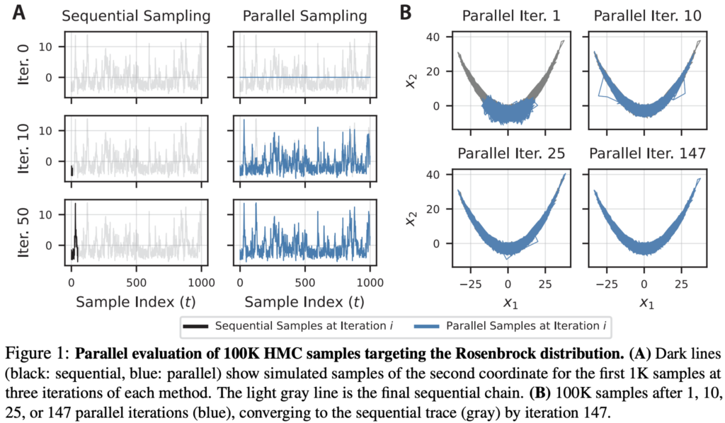
The above graph shows what’s happening.

“Sequential Sampling” is when they run HMC on this example. The gray line shows the trajectory or sequence of simulation draws. (Here they just do one chain to demonstrate the idea, but later in the paper they talk about the benefits of simulating multiple chains.) The trajectory is a random vector, but it can be thought of as deterministic, conditional on the sequence of random numbers that is used to do the jumping and make the accept/reject decisions.

Here’s the idea: Given the input sequence of random numbers, the goal is to compute that trajectory. But rather than doing it the usual way, by running HMC, they do it by starting with an initial guess–here, the flat or constant trajectory shown as the horizontal line of the top graph above in the “Parallel Sampling” column–and then moving the points around until they reach the correct trajectory. This can be done because the correct trajectory is Markovian (in this case, first-order Markov), and the value at each time point from t=1 through t=1000 is a known deterministic function of the value at time t-1 and the set of input random numbers corresponding to that iteration. They write this as s_t = f_t(s_{t-1}), where f_t is that deterministic function, and the random numbers for time t are implicitly included in f_t.

Each iteration of the parallel algorithm is a step in which the values of the trajectory at each point are jiggled up and down in an attempt to make each s_t as close as possible to f_t(s_{t-1}), for each t. The beauty of this algorithm is that these updates can be done locally, so you can do them in parallel. It turns out that this can be done in O(log(T)) ticks of wall time. The update requires O(T) computations but with enough processors the parallelism saves lots of time.

When does this make sense? I know next to nothing about parallel computing, but apparently it can be done on GPUs, and there are now programming languages that can distribute the computing steps.

There are lots of details that make this work, including using autodiff on the functions f_t.

Discarding bad approximations in the middle of the chain?

Here’s something I noticed about their example.

Look at Figure B above: it shows that after 147 iterations of the parallel updating, the computation has reached the correct values of the chain for this set of input random numbers. But what about after 10 iterations? It’s pretty damn close already! There seem to just be 4 or 5 points that are in the wrong place.

So here’s my question. Could there be a way, if you want to stop early, to identify those bad points and throw them out?

Usually when we’re doing HMC, you have to keep the whole chain or throw it all out, or maybe you keep running it and you throw away the initial part that hasn’t completely warmed up. But in this new algorithm, the entire chain is a static target, so it seems that it might be possible to just throw away a few bad iterations in the middle.

At first this idea might seem hopeless: if you don’t know the final answer, how would you know which points to throw out? But we can compare each s_t with f_t(s_{t-1}), so maybe just take the points where the discrepancy is large and toss them?

As a start, I’d be interested in how things work with the example shown above. Do the bad points in parallel iteration 10 correspond to large values of |s_t – f_t(s_{t-1})|? If so, maybe there’s something we can do here! Nothing stopping us from continuing to run all the way to parallel iteration 147 or whatever, but in the meantime maybe we can do better along the way.

A counterintuitive example where a strong prior pulls an estimate in the wrong direction–and how to see the problem

It goes like this. We start with a simple linear regression. In the Stan code we first simulate data given the true parameter values and then express the model:

data {
  int N;
  real a_true, b_true, sigma_true;
}
transformed data {
  vector[N] x;
  vector[N] y;
   for (n in 1:N) {
    x[n] = uniform_rng(0, 50);
    y[n] = normal_rng(a_true + b_true * x[n], sigma_true);
  }
}
parameters {
  real a, b
  real<lower=0> sigma;
}
model {
  for (n in 1:N) {
    y[n] ~ normal(a + b * x[n], sigma);
  }
}

And here are the input data:

{
  "N": 100,
  "a_true": 20,
  "b_true": 0.8,
  "sigma_true": 15
}

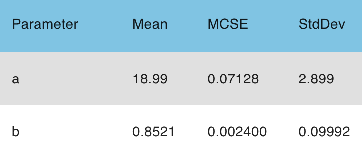
We compile and run it in Stan Playground, setting the seed to 123, and here are the results:

This all seems reasonable. The true values of a, b, and sigma are 20, 0.8, and 15, and the estimates are 19.0 +/- 2.9, 0.85 +/- 0.10, and 15.5 +/- 1.2.

Now let’s try throwing in a prior. I’m gonna use my default prior for parameters on unit scale:

  a ~ normal(0, 1);
  b ~ normal(0, 1);
  sigma ~ exponential(1);

This goes into the model block of the above Stan program.

Before going on, let me point out that the parameters of this problem are not on unit scale. By “unit scale,” I mean, “being drawn from a distribution with scale that is of order 1,” and a_true = 20 here. Not unit scale at all! Also, sigma_true = 15, but this will be less of an issue because the exponential prior is much weaker than the normal in the tail.

So, yeah, this is a terrible prior. But, y’know, that happens. Not on purpose (usually), but we’re all busy and sometimes we apply models that don’t make sense or don’t fit the data, or both.

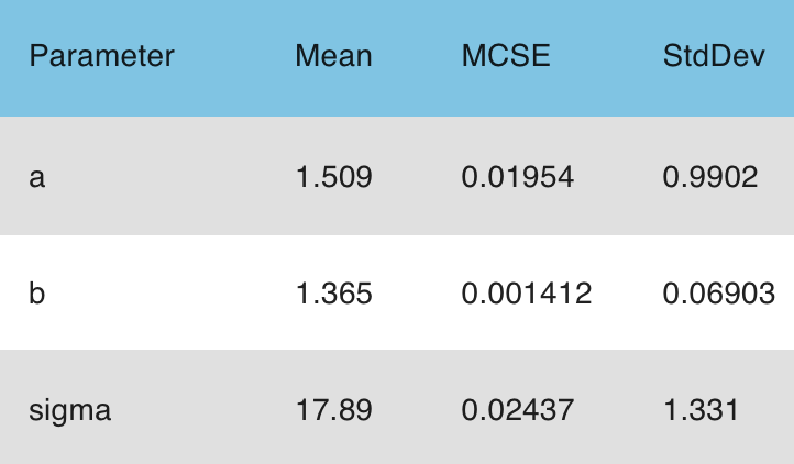
So let’s see what happens with this strong prior.

Actually, we kind of know what to expect. The likelihood is centered at (a, b, c) = (19.0, 0.85, 15.5), and the prior mode is at (0, 0, 0), so we expect the parameter estimates all to be pulled toward zero. Especially the intercept, a, since the prior for a is much stronger than the likelihood. And it’s a linear normal model so the posterior should be pulled smoothly toward the prior, not the sort of funny stuff that would happen with a Cauchy prior, say.

But let’s run it and see what happens. Here goes:

Let’s look at each parameter:
– The estimate for “a” has gone from 19.0 to 1.7: So, yeah, the prior was strong, it pulled the estimate almost all the way to the prior mode of 0.
– The estimate for “b” has gone from 0.85 to 1.4: Wha….?? It got pulled away from the prior!
– The estimate for “sigma” has gone from 15.5 to 16.5: Again, it got pulled in the wrong direction!

What’s going on here?

The key to understanding this problem is to realize that, although the three parameters a, b, and sigma are independent in the prior distribution here, they’re strongly dependent in the likelihood.

So let’s talk through what’s happening.

First, the prior for “a” is very strong, so the intercept is pulled almost all the way to 0.

Second, look at the data. The predictor x ranges from 0 to 50, and the true regression line is y = 20 + 0.8x, so if you grab the line at x=0 and pull it down from y=20 to y=0, while still trying to go through the data, you’ll increase the slope. Just draw the scatterplot and you’ll see what I mean.

So the strong prior on “a” causes the estimated slope to go up. Also there’s a prior on “b” that pulls the slope toward 0, but it’s a weak prior relative to the likelihood (recall that the likelihood-based estimate of b had a standard error of 0.1), so it doesn’t have much effect. The net effect of the joint prior is to increase the slope of the fitted line, thus pull the estimate of b away from 0 in this case.

Finally, the new line doesn’t fit the data so well–that’s what happens when you move away from the maximum likelihood estimate, the fit gets worse!–and so the estimate of sigma goes up. Again, there is a prior on sigma that pulls its estimate toward zero, but it’s not as strong as the signal from the data telling us that the fit is getting worse.

We can see this even more clearly by removing the priors on b and sigma, so that all we have is the prior on the intercept, a:

data {
  int N;
  real a_true, b_true, sigma_true;
}
transformed data {
  vector[N] x;
  vector[N] y;
   for (n in 1:N) {
    x[n] = uniform_rng(0, 50);
    y[n] = normal_rng(a_true + b_true * x[n], sigma_true);
  }
}
parameters {
  real a, b;
  real<lower=0> sigma;
}
model {
  a ~ normal(0, 1);
 // b ~ normal(0, 1);
 // sigma ~ exponential(1);
  for (n in 1:N) {
    y[n] ~ normal(a + b * x[n], sigma);
  }
}

And here’s what happens:

So, yeah, the inference for “b” is about the same, “sigma” gets pulled up even more, and “a” gets pulled even more toward zero. That last bit makes sense too: in the model with informative priors on all three parameters, the priors on b and sigma have the effect of somewhat decreasing the amount that the intercept can be pulled down to zero.

Lessons from this example

First, put your parameters on unit scale so that you won’t accidentally use priors that are so contrary to the data. At this point you might say that you don’t know anything about your parameters so you can’t put them on unit scale. But I disagree! In every application I’ve seen, we have some sense of the scale of the effects and adjustments in the model. If you don’t have this information–if you’re flying blind, as happens when you’re developing default software–then there should be a way to scale the parameters based on the data. That’s how we do things in rstanarm, as discussed in Section 9.5 of Regression and Other Stories.

Second, plot the data and fitted model. Check the fit of the model to the data! You’re under no obligation to stick with a model that clearly doesn’t fit.

Third, experiment! As shown above, you can learn a lot by perturbing the model and re-fitting. No need to just stare at your code and your computer output to try to figure out what is happening. You can and should use experimentation as a regular tool.

A Stan transpiler in Julia!

Nikolas Siccha writes:

I got inspired by Bob’s latest blog post to bring your attention to this code generation tool. It’s currently supremely buggy and only really usable by myself – but it may still be interesting for you to see, as it IMO solves many of Stan’s “problems.”

“Supremely buggy and only really usable by myself” . . . that describes lots of the software that I write!

Follow the link and here’s what you see:

StanBlocks.jl (Stan backend)

Brings Julia syntax to Stan models by implementing a (limited) Julia to Stan transpilation with many caveats. See test/slic.jl for implementations of a few simple posteriordb models and see src/slic_stan/builtin.jlfor a list of built-in functions and examples of user defined functions.

Current features include

  • activity analysis (automatically determines what is data, transformed_data, parameters, transformed parameters, model, or generated quantities),
  • automatically inferred types, shapes and constraints – including for user defined functions (including the function arguments, function body, and function return type),
  • automatic posterior pointwise likelihood and predictive generation,
  • (variadic) user defined functions,
  • higher order (user defined) functions (such as map, broadcasted, sum and more),
  • sub models,
  • post-hoc model adjustment,
  • named tuples,
  • (approximate) automatic code formatting à la Blue,
  • and more.

Upcoming features include, in order of priority and estimated arrival,

  • easy runtime assertions (like Julia’s @assert) – and support for other macros,
  • model docstrings,
  • custom types (for method dispatch – this would help with more “Julia-style” broadcasting, e.g. via Ref),
  • closures via Julia’s Do-Block Syntax (to make within chain parallelization via reduce_sum less painful),
  • lower transpilation runtimes (currently, transpilation can sometimes take longer than compilation – there is currently at least one algorithmic inefficiency on top of the systemic implementation inefficiency),
  • a much better user experience,
  • more and better tests,
  • keyword arguments,
  • default arguments,
  • inlining (to reduce potential runtime overhead),
  • easier custom parameter transformations (going from sampler parametrization to user parametrization – aka as constraining),
  • array comprehensions,
  • a more complete (and more correct) coverage of built-in Stan functions,
  • better name resolution (currently user defined functions or sub models have to be defined in Main),
  • functions that mutate their arguments (solved via inlining),
  • and more.

Almost anything that’s possible in Julia should be possible to be transpiled to Stan. Of course, unless Stan is much faster than Julia (+Mooncake or Enzyme) for the model in question, just sticking to Julia comes with many advantages.

Features which I am on the fence about, but currently not planning to implement:

  • a Julia backend,
  • target += statements,
  • top level control flow,
  • top level mutability,
  • getting rid of superfluous parentheses.

Features which are NOT planned:

  • (automatically) transpiling Julia functions which have not been defined via @deffun.

The earn_height.stan model below becomes

using StanBlocks
import PosteriorDB, StanLogDensityProblems, JSON

# Get data from PosteriorDB
pdb = PosteriorDB.database()
post = PosteriorDB.posterior(pdb, "earnings-earn_height")
(;earn, height) = (;Dict([Symbol(k)=>v for (k, v) in pairs(PosteriorDB.load(PosteriorDB.dataset(post)))])...)

# Model definition
earn_height_model = @slic begin 
    beta ~ flat(;n=2)
    sigma ~ flat(;lower=0.)
    earn ~ normal(beta[1]+beta[2]*to_vector(height), sigma)
end
# Not compiled yet
earn_height_posterior = earn_height_model(; earn, height)
# Prints the Stan model code
println(stan_code(earn_height_posterior))
# Compiled (requires StanLogDensityProblems and JSON)
earn_height_problem = stan_instantiate(earn_height_posterior)

I don’t quite get that code at the end, but then again I don’t speak Julia.

One reason I think this is cool is that Julia and Stan started at the same time! Both projects were originally supported by a Department of Energy grant that funded Alan Edelman and me to hire postdocs and programmers. Alan’s group built Julia; we built Stan. Thanks, Bob, Matt, Daniel, and everybody else who did this!

Stepping back, it’s good to be able to go between languages and not be stuck in just one framework. We wrote Stan for two reasons:

1. To be able to easily and flexibly express Bayesian models and fit them to data.

2. To be able to perform statistical workflow, which includes fitting multiple models, postprocessing inference, plotting data and fitted models, etc.

For step 2, it was absolutely necessary for Stan to link smoothly to general-purpose computing environments such as R and Python, which is why we built rstan and pystan (which have since mostly been replaced by the lighter interfaces cmdstanr and cmdstanpy; thanks, Jonah, Mitzi, and everybody else who did this!). You can also run Stan from Julia. What Niko is doing here is going beyond that in allowing some sort of improved version of Stan that can be written in Julia, which seems like it could be really useful.

Beyond all this, as a scholar I’ve always tried to avoid any territorial attitude. I’ve just seen this too often, with researchers who have some method or another and are out there dissing the competition. OK, don’t get me wrong here, I’m happy to diss, when it’s appropriate, but not just cos it’s competition. Science isn’t a competition; we’re all in this together.

So, yeah, Stan is great. I love Stan, and I use it. I eat my own dogfood. But the purpose of Stan is Bayesian workflow. And if Stan can be helpful to Bayesian workflow in other ways, that’s great.

The Mets are hiring

Sam Saskin writes:

I’m reaching out because we are hiring for a couple of jobs on the Mets analytics team and I was wondering if you’d be willing to share the job postings on your blog. The two positions (posting links below) are Senior Data Scientist, which would be a match for anyone looking for a full-time position, and Data Science Intern, which would be a match for current students (either undergraduate or graduate) who would be interested in spending a summer working with our team. I really appreciate the assistance, as we’ve had a lot of luck finding great candidates through visibility on your blog in the past.

Also if you have a 100 mph fastball they might be able to find a place for you somewhere in the organization.

Pinning the group-level variance parameters to speed computation for hierarchical models

In case you don’t know about the Stan Forums, let me just tell you that it’s a great online space for discussions about applied statistics and computing. All sorts of things come up.

Today we had a discussion about challenges of fitting big hierarchical models, where I wrote:

1. I often recommend pinning the group-level variance parameter or covariance matrix to a pre-chosen value based on subject-matter information. Often the inference isn’t super-sensitive to this group-level variance, as long as it’s not so small that it causes all the estimates to disappear to zero and not so large that the estimates are wildly noisy.

I’ve toyed with the idea of making this a more formal procedure, for example drawing 10 values of the set of variance parameters from a prior, then using these to run 10 fast inferences (could be MCMC or even just plain old optimization and Laplace approx), then averaging over them using stacking. I think this could work, but I’ve never actually tried it, let alone evaluated the idea. It’s a research idea!

2. Sometimes we do use gamma priors for group-level variance parameters. The gamma prior with 1 or more degrees of freedom has the pleasant property of being zero-avoiding, which is especially helpful when doing marginal maximum likelihood, as we discuss in our 2013 paper: https://sites.stat.columbia.edu/gelman/research/published/chung_etal_Pmetrika2013.pdf or for covariance matrices (using the Wishart, _not_ inverse-Wishart) prior for cov matrix in our 2014 paper: https://sites.stat.columbia.edu/gelman/research/published/chung_cov_matrices.pdf

3. Another thing that’s worked well for me is to use Pathfinder to get starting values. It varies, but sometimes Pathfinder runs very fast and then we can jointly estimate all the parameters and not worry so much about the funnel.

I’m sharing this here partly because it might be useful to some of you and partly because it includes a research idea.

Simulating from and checking a model in Stan: It’s so easy in Stan Playground–it just runs on your browser!

When building models, it’s helpful to check our understanding by simulating fake data and seeing if the fitted model can recover the true underlying parameters. And it’s so easy to do in Stan!

See above–I just did a simple example in Stan Playground. (Thanks, Brian!) The code’s kind of ugly because I specified the true parameter values in the transformed data block Stan code rather than calling them as data; on the upside the whole thing is then in one program.

This is not the same as full simulation-based calibration checking (SBC). In SBC you draw the true parameter values from the prior, repeat the entire process in parallel many times, and then check the average coverage of posterior inferences with respect to the true parameter values, averaging over the prior. Here I’m just running one simulation and setting the true parameter values just once. It’s a kind of quick-and-dirty SBC which can still be useful in catching problems such as nonidentified models or poor mixing.

And it’s so easy to do! Whenever you fit a model, you should be checking it on fake data.

I was doing the above example because I wanted to quickly check for one of the exercises I’m writing for the forthcoming Bayesian Workflow book.

P.S. Here’s the code for the above example if you want to try it yourself:
Continue reading

Seven-parameter drift-diffusion pdfs and cdfs now in Stan

This post is from Bob.

Drift-diffusion models

Whew. The cdf function for the seven-parameter drift-diffusion model was just merged. The pdf was merged a few months ago. This is a big deal. These pdfs and cdfs are used for in decision-time models in cognitive psychology. There’s a really nice illustration through NLM on nih.gov. The basic idea is that you have a binary task like deciding if an image is red or blue. The data being recorded is time to decision and the decision being made. The underlying generative model is a continuous Wiener diffusion process that has a lag time to get started before drifting with some bias toward opposing decision boundaries. The decision is determined by when it crosses a boundary and which one it crosses (see the illustration). The cdf is important when the task ends before a decision is made, giving you censored observations, which require cdfs or truncated pdfs to implement.

The first time I saw this model being applied was by Bruno Nicenboim and Shravan Vasishth (psycholinguists at Potsdam at the time, though Bruno has since moved to Tilburg) about six or eight years ago. At that point, it took Stan a month or so to fit the model (yes, that’s a month, not a typo)—you may know them as two of the three authors of the really wonderful book, Introduction to Bayesian Data Analysis for Cognitive Science (2025, CRC), which, in its final chapter, covers accumulator models of which the drift-diffusion model is one form. Now these models are very fast in Stan with the new built-in functions.

The pull requests and engineering challenge

Hats off to Franziska Henrich, a cognitive psychologist and Stan developer at the University of Freiburg, aka GitHub user Franzi2114, for writing the code and bearing with Steve Bronder’s hundreds of comments and fixes and my final round of a hundred or so change requests. You can see all the gory details in the discussions around the pull requests and in the code itself.

These pair of functions were perhaps the two hardest functions to get into Stan for a myriad of reasons. The most challenging obstacle beyond the inherent complication of the functions themselves is that our testing framework for densities can’t handle seven-parameter densities. So all the tests had to be projected into subsets of parameters (and seven choose four or five or whatever it was led to a lot of tests). A further difficulty is that to make the arithmetic stable, the code branches all over the place (see the Hartmann and Klaeur article linked below), which also complicates testing.

Some academic background

In addition to Vasishth et al.’s book chapter, there is a vast literature on drift-diffusion models in cognitive psychology and elsewhere. Most relevantly, Franziska wrote an open-access article about the model and the Stan implementation.

Luckily, Hartmann and Klauer provided the derivatives in a previous (closed-access) article.

As is often the case, you can find a pdf through Google Scholar. It’s a daunting pile of mathematics that puts the “M” in “mathematical psychology.” Luckily for us, the authors published an R implementation in package WienR on CRAN (the name is because it’s the Wiener diffusion model underlying the process), which Franziska could use for testing.

Coming to the Stan language next release

We just put out a new Stan release, so we have plenty of time to get the language wrappers around the math library functions before the next release of Stan. Ideally, we’ll also have a User’s Guide chapter with examples of how to use them. We’re always open to new *User’s Guide* chapters about models or methodologies in wide use, and as you can see from this example, we take pull requests, which go down much more easily with the User’s Guide.