I just read this compelling op-ed by Brendan Ballou, “One Man Stole $660 Million. He’ll Never Pay It Back,” which tells the story of several brazen white-collar criminals who avoided prosecution for federal crimes by the simple expedient of bribing the president of the United States. Ballou argues, though, that there could still be ways of catching these guys:
In a world where the Department of Justice and the president are either indifferent to or actively support rich criminals, what can be done? Fortunately, there is a range of legal tools that ordinary citizens can use to pursue civilly the sort of corruption that would ordinarily be prosecuted criminally.
The shareholders potentially cheated by Mr. Wiederhorn could sue the Trump inaugural committee under the federal civil RICO law — written to destroy the Mafia — for seemingly helping to secure Mr. Wiederhorn’s freedom. Companies that follow the law can sue rivals, like Binance, that do not, under California’s Unfair Competition Law. And investors scammed by Mr. Milton can sue the political committees he donated to if they were “unjustly enriched” by his scheme. . . .
When regular citizens can’t act themselves, they can pressure their local prosecutors to do so. Recall Mr. Homan’s $50,000 in cash from undercover F.B.I. agents. This Justice Department may not continue the investigation. But Mr. Homan’s personal business is headquartered in Virginia, and it would be awfully interesting to find out whether Mr. Homan reported that money on his state tax returns. If he didn’t, he may well have committed a crime. . . .
He concludes:
Criminals and government officials are barely hiding their schemes, and their brazenness is meant to make us feel helpless, to think that nothing can be done. That is false. We already have the legal tools to fight corruption. We just need to use them.
This is inspirational and I hope someone does all of this.
My point in the present post is that getting justice can require a lot of effort.
Here’s an example. The other day I was talking with someone about research fraud, and he characterized the Michael Lacour story as the biggest scandal ever in political science. I disagreed. It was my impression that Lacour had been forgotten (here’s some background), but what about the time that the American Political Science Association gave an award to a plagiarized book? Here’s the story. I’d never heard of any of the people involved in that episode, but it incensed me that APSA had done this.
I wasn’t the only angry person. Indeed, I’d heard about the Frank Fischer case from Alan Sokal, who’d emailed an academic official at Rutgers University, where the plagiarist worked, but there was no useful response. So I decided to take a whack at it. I sent off this email to the people on the committee that had given that award:
Dear APSA Public Policy Section:
I learned recently that you gave your 2017 Aaron Wildavsky Enduring Contribution Award to Frank Fischer for his 2003 book Reframing Public Policy. I was surprised to hear this, given that the book appears to have plagiarized material. For background, see this document by Krešimir Petković and Alan Sokal:
https://chronicle-assets.s3.amazonaws.com/5/items/biz/pdf/plagiarism_fischer.pdf
and this note by Petković:
https://chronicle-assets.s3.amazonaws.com/5/items/biz/pdf/Petkovic_Experiment_with_CPS.pdf
and this news article for further background:
https://www.chronicle.com/article/alan-sokal-takes-aim-at-an/124969
Petković, a political science graduate student in Croatia, found places in Fischer’s 2003 book where he had used materials from previously published work by others without giving full attribution. In addition to copying without attribution (as Petković writes, Fischer mentions the book he copied from, but nowhere near the copied passage), Fischer also makes mistakes such as misspelling authors’ names and reproduces errors that arose in the original sources.
Two of the works from which Fischer copied in his 2003 book without appropriate attribution are:
Majone, Giandomenico, 1989. Evidence, Argument, and Persuasion in the Policy Process. New Haven: Yale University Press.
Walsh, David, 1972. Sociology and the Social World. In: Filmer, Paul, Phillipson, Michael, Silverman, David and Walsh, David, New Directions in Sociological Theory. London, Collier-Macmillan: 15-35. [Also published by MIT Press, Cambridge, Mass., 1973.]
I am not an expert in this area and have no intention of pursuing any formal process here. Indeed, I am not even a member of APSA. However, I am a political scientist and, as such, am distressed to see APSA promoting plagiarism.
My recommendation is that you retract the award. If that is too difficult, one thing you could do is retroactively also give this award to Majone (1989) and Walsh (1972). It does not seem fair that they did the work and someone else gets the award, no? I do not know Prof. Fischer and am making no judgment regarding the quality of his writing. It may be that it is indeed an enduring contribution to the field; if so, all authors of this enduring contribution should be recognized.
Yours,
Andrew Gelman
Professor, Department of Statistics
Professor, Department of Political Science
Columbia University, New York
P.S. I have also cc-ed the members of APSA’s Committee on Professional Ethics, Rights, and Freedoms.
From APSA’s guide to professional ethics:
“7. Political scientists, like all scholars, are expected to practice intellectual honesty and to uphold the scholarly standards of their discipline.
7.1 Plagiarism, the deliberate appropriation of the work of others represented as one’s own, not only may constitute a violation of the civil law but represents a serious breach of professional ethics.
7.2 Departments of political science should make it clear to both faculty and students that such misconduct will lead to disciplinary action and, in the case of serious offenses, may result in dismissal.”
A few months later I followed up:
Hi all. I was just wondering what happened with this. As I wrote last year to **, I am not submitting a formal grievance or complaint. I just wanted to let the committee be aware of this situation so that they can have the opportunity to fix it.
So I was interested to find out how things have progressed, as it seems to be an embarrassment to APSA to have given a major award for a book with plagiarized material!
Andy
After several months I hadn’t heard back from the committee so I pinged them in June. A couple weeks later they got back to me and said they couldn’t do anything because it had not been submitted as a formal complaint.
Fair enough. I didn’t think it would be right for me to file the complaint myself, given that I’m not at all knowledgeable about this area of political science.
Meanwhile, the books that had been plagiarized, Majone (1989) and Walsh (1972), never got that award. Doesn’t seem fair to me!
Anyway, my point is that it takes work to pursue these things, and it’s more my inclination to point out the problem than to go through the political and administrative steps needed to rectify the problem.
I’m not dissing “the political and administrative steps”–I have a lot of respect for people who can do these things!–it’s just not something that I’m good at.
Here’s another example. I once had a colleague who plagiarized my work. When I realized what was going on, I was stunned. But then, looking back, I realize that I’d been warned of this behavior years earlier, indeed my memory flashed back to a time that I’d seen something else he’d plagiarized from me, and I’d just kind of filed that image in my mind and forgotten it. My collaborator and I had a good thing going, and, hey, nobody’s perfect, so it was easier to look away. When I confronted him about the plagiarism–this was a long time ago–he kind of wriggled around, saying that he didn’t want to share credit with me on the project I’d been working on with him–at one point I was dictating formulas to him over the phone–but we could jointly write a separate article on the topic. This just pissed me off, but, ultimately, he won, in the sense that he correctly calculated that I was rational enough not to want to get involved in a major scandal early in my career. Yes, he’s the one who would’ve looked bad had I raised a formal complaint, but it wouldn’t have done my reputation any favors to be seen as a complainer. Also, though, I won, in that I stopped my involvement in this project and I moved on to better collaborators.
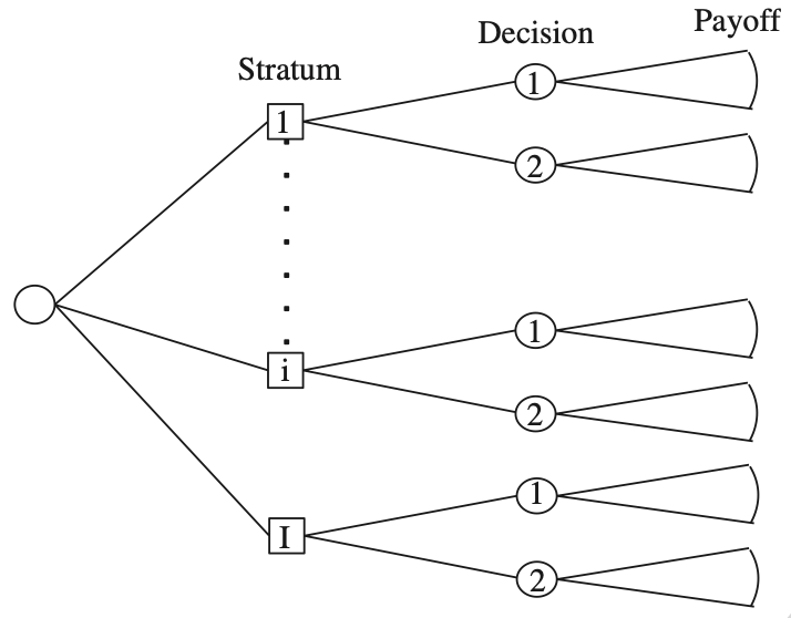
The episode bothered me (which is why I keep talking about it), but my cost-benefit analysis led to the decision to not file a formal complaint. That’s the decision-theory analysis. The game-theory analysis is that my colleague could see ahead to the next move: he know I was rational and that it would be a net loss to me to make a fuss about his actions, and I expect that this minimax analysis led him to the conclusion that he’d be safe in plagiarizing me. Yes, he was taking a risk to his reputation in doing so, but it was a calculated risk, in his mind less than the expected benefit to his reputation of taking full credit for this part of our joint research.
What should be done?
I’m not sure. In academic scandals, maybe it’s best just to move on. So what if some obscure political scientist got some award that he didn’t deserve? So what if some researcher publishes substandard work because he decides to not credit a collaborator? Worse things happen every day in academia. Indeed, if you want to talk about the worst scandal in modern political science, I might give the nod to Samuel Huntington’s book, The Clash of Civilizations and the Remaking of World Order, not because of plagiarism or anything like that, but just because arguably it’s had a large and malign influence in the world. Given all the problems in social science, plagiarism is the least of our concerns. So, although it annoys me, ultimately I think the appropriate strategy is to just let it happen, to talk about it but not to worry about seeking justice.
When it comes to business and government corruption, though, I agree with Ballou that something should be done. Legislatures should be writing laws, local and state governments should be prosecuting, lawyers should be suing, etc. These guys are stealing, giving and taking bribes . . . this is the kind of thing that degrades the entire economic and political system.
So, again, I hope some people make some of the moves that Ballou recommends. They should just be aware that it will take a lot of effort and persistence.