Lots is written on this blog about “Poststratification”. Andrew addresses it formally with a “Mister“. But when I learned it from Alan Zaslavsky’s course it was casually just “Poststratification”. At the time it sounded to me like damage control after we forgot to stratify.

- “Stratification” so that your sample has the same distribution for variables X as in the population: divide the population into strata (i.e. groups) based on X. Then take a sample in each stratum proportional to its size.
- “Post“: divide the population into strata only after the sample is already selected.
(As Raphael Nishimura and Andrew Gelman pointed out in the comments below, stratification has other uses !)
Fancy graphics from a DOL video I worked on:

How can Poststratification help ?
Suppose we want to estimate E[Y], the population mean. But we only have Y in the survey sample. For example, suppose Y is voting Republican. We can use the sample mean, ybar = Ehat[Y | sample] (I don’t know how to LaTeX on this blog).
But our sample mean is conditional on being sampled. And what if survey-takers are more or less Republican than the population ? As Joe Blitzstein teaches us: “Conditioning is the soul of statistics.” Conditioning on being sampled might bias our estimate. But maybe more conditioning can also somehow help us ?! Joe taught me to try conditioning whenever I get stuck.

If we have population data on X, e.g. racial group, then we can estimate Republican vote share conditional on racial group E[Y|X] and aggregate according to the known distribution of racial groups, invoking the law of total expectation (Joe’s favorite): E[Y] = E[E[Y|X]]. So if our sample has the wrong distribution of racial groups, at least we fix that with some calibration. Replacing “E” with estimates “Ehat”, poststratification estimates E[Y] with E[Ehat[Y | X, sample]].
When our estimate of E[Y|X] is the sample mean of Y for folks with that X, the aggregate estimate is classical poststratification, yhat_PS. When our estimate of E[Y|X] is based on a model that regularizes across X, the aggregate estimate is Multilevel Regression (“Mister“) and Poststratification, yhat_MRP. Gelman 2007 shows how yhat_MRP is a shrinkage of yhat_PS towards ybar.
Which estimate is best for estimating E[Y] ? ybar, yhat_PS, or yhat_MRP ?
As Kuh et al 2023 write:
it is not individual predictions that need to be good, but rather the aggregations of these individual estimates.
A parallel approach is through simulation studies—for greater realism, these can often be constructed using subsamples of actual surveys—as well as theoretical studies of the bias and variance of poststratified estimates with moderate sample sizes.


“Stratification” = divide the population into strata (i.e. groups) based on some variables … for representativeness. |
… seems confusing and departs from normal statistical probability sampling — by subjectively manipulation of the gathered Sample and ‘specific’ Population being sampled.
I don’t love that definition either. Both because I *really* don’t like the notion of “representativeness”, but also because this is just a specific use of stratification, i.e., allocate the sample proportionately to the population across the strata with an expectation of gains in precision. But there is more of stratification than this.
Thanks, Raphael !
Great point, which Andrew echos below. Stratification has more uses than trying to gain precision for estimating a population average.
Curious to hear more about your objections to the notion of “representativeness”.
It’s a variation of probability sampling (EPSM) but it requires detailed knowledge of the sampling frame prior to selection, which is only possible in specific cases. You have to adjust the standard error estimations because you’re guaranteed not to have a sample that contains members of just one group.
Shira:
Thanks as always for the posts. Regarding definitions:
1. As Raphael says, stratification in sampling is not always done with the goal of representativeness. Often a stratum will be purposely oversampled. This especially comes up when you’re sampling organizations rather than people. You can have a stratum with a small number of large organizations that are likely to be included in the sample and then strata with many small organizations, each with low probability of inclusion. You can even have a certainty stratum in which everything gets sampled.
2. In many settings, stratification is not a choice: you don’t have a single sampling frame, or for reasons of practicality you will do a separate sampling process within each stratum.
3. One way I sometimes describe poststratification is the analysis of unstratified sample data as if they were stratified.
4. In modern poststratification (MRP or RPP–that is, multilevel regression and poststratification or, more generally, regularized prediction and poststratification), we are still estimating the population within each stratum, but these estimates are themselves constructed through model fit to all the sampled data. So it doesn’t look like a classical stratified estimate. That said, these same procedures can be used to analyze stratified data too. For the purpose of the analysis, it doesn’t really matter whether the sampling procedure was stratified or not!
5. I’d also point everyone to our new paper on MRPW (MRP with sampling weights), but Columbia’s server still seems to be down. Once the server is up again, you can find it at this page.
If it is done for oversampling purposes then you would need to apply weights when analyzing the combined data. Another way stratification is interesting is if you see it as a kind of limiting case of cluster sampling in which all the clusters are included.
I often have students use this https://cress.soc.surrey.ac.uk/samp/index.html and compare the results with 10 samples for each of the methods. Stratified random sampling almost always wins on estimates but loses on how much it costs.
Thanks, Andrew !
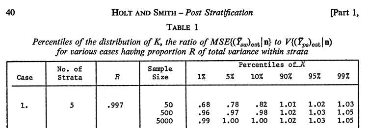
1. Indeed, Holt & Smith 1979 begins highlighting at least 2 purposes: “STRATIFICATION is one of the most widely used techniques in sample survey design serving the dual purposes of providing samples that are representative of major sub-groups of the population and of improving the precision of estimators.”
2. yup ! I think this was the case in our Millennium Village Project ? There were budgets and sampling frames per country.
3. that’s a nice description !
4. Holt & Smith 1979 introduction also says: “In one way post stratification is potentially more efficient than stratification before selection since after sampling the stratification factors can be chosen in different ways for different sets of variables in order to maximize the gains in precision.”
5. Looks like the server is back up ! Thanks for pointing me to this paper. Does it compare these MRP(W) also to classical poststratification and no poststratification ?
The most common calculation method for this is probably by using survey weights. Eg in this case, if you think non-response rates differ by race, you would adjust the design weights to compensate for this. It looks like this is the same as the post-stratification calculation you describe.
When there are multiple calibration variables, however, there is not a unique way to calculate these weights. Are there links between the literature on creating survey weights and the MRP approach?
With post-stratification there *is* a unique way to calculate the weights. Post-stratification is the special case where you just match observed and expected numbers for each cell in a partition of the sample space (a ‘saturated model’, sort of), so all the ways to adjust weights turn out to be the same: estimating sampling probabilities (with any link function) or calibration with any distance metric.
Often with multiple variables you can’t afford post-stratification because there would be too many post-strata, and that’s when there are all the choices.
Your last sentence is approaching what I was thinking of. Researchers (or data providers) often have multiple calibration variables, but not the intersection of these variables. So, iterative methods are used to adjust weights to satisfy all the calibration variables simultaneously. But, there are tradeoffs. If calibration variables are inconsistent, you can end up with very high weights on individual cases. So, I’m wondering if the MRP approach is a better approach here.
Thanks, Thomas !
In your book “Complex Surveys” p.142 you write:
In the comment you’re saying that when X are a complete cross-classification of a set of categorical variables, then all d( , ) give the same weights ? Is this “obvious” ?