It goes like this. We start with a simple linear regression. In the Stan code we first simulate data given the true parameter values and then express the model:
data {
  int N;
  real a_true, b_true, sigma_true;
}
transformed data {
  vector[N] x;
  vector[N] y;
   for (n in 1:N) {
    x[n] = uniform_rng(0, 50);
    y[n] = normal_rng(a_true + b_true * x[n], sigma_true);
  }
}
parameters {
  real a, b
  real<lower=0> sigma;
}
model {
  for (n in 1:N) {
    y[n] ~ normal(a + b * x[n], sigma);
  }
}
And here are the input data:
{
  "N": 100,
  "a_true": 20,
  "b_true": 0.8,
  "sigma_true": 15
}
We compile and run it in Stan Playground, setting the seed to 123, and here are the results:
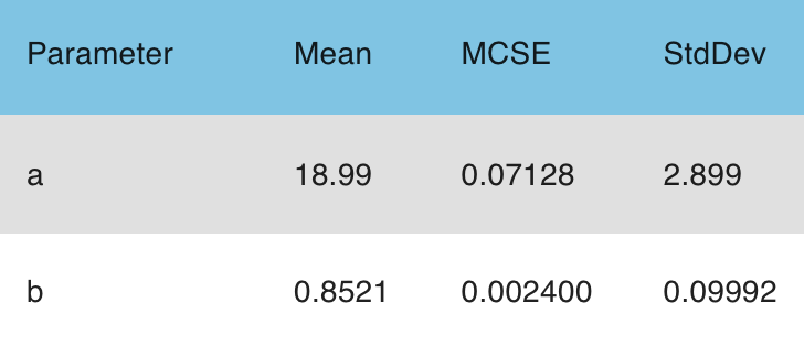
This all seems reasonable. The true values of a, b, and sigma are 20, 0.8, and 15, and the estimates are 19.0 +/- 2.9, 0.85 +/- 0.10, and 15.5 +/- 1.2.
Now let’s try throwing in a prior. I’m gonna use my default prior for parameters on unit scale:
  a ~ normal(0, 1);
  b ~ normal(0, 1);
  sigma ~ exponential(1);
This goes into the model block of the above Stan program.
Before going on, let me point out that the parameters of this problem are not on unit scale. By “unit scale,” I mean, “being drawn from a distribution with scale that is of order 1,” and a_true = 20 here. Not unit scale at all! Also, sigma_true = 15, but this will be less of an issue because the exponential prior is much weaker than the normal in the tail.
So, yeah, this is a terrible prior. But, y’know, that happens. Not on purpose (usually), but we’re all busy and sometimes we apply models that don’t make sense or don’t fit the data, or both.
So let’s see what happens with this strong prior.
Actually, we kind of know what to expect. The likelihood is centered at (a, b, c) = (19.0, 0.85, 15.5), and the prior mode is at (0, 0, 0), so we expect the parameter estimates all to be pulled toward zero. Especially the intercept, a, since the prior for a is much stronger than the likelihood. And it’s a linear normal model so the posterior should be pulled smoothly toward the prior, not the sort of funny stuff that would happen with a Cauchy prior, say.
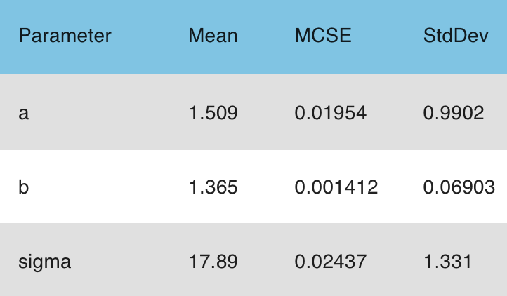
But let’s run it and see what happens. Here goes:

Let’s look at each parameter:
– The estimate for “a” has gone from 19.0 to 1.7: So, yeah, the prior was strong, it pulled the estimate almost all the way to the prior mode of 0.
– The estimate for “b” has gone from 0.85 to 1.4: Wha….?? It got pulled away from the prior!
– The estimate for “sigma” has gone from 15.5 to 16.5: Again, it got pulled in the wrong direction!
What’s going on here?
The key to understanding this problem is to realize that, although the three parameters a, b, and sigma are independent in the prior distribution here, they’re strongly dependent in the likelihood.
So let’s talk through what’s happening.
First, the prior for “a” is very strong, so the intercept is pulled almost all the way to 0.
Second, look at the data. The predictor x ranges from 0 to 50, and the true regression line is y = 20 + 0.8x, so if you grab the line at x=0 and pull it down from y=20 to y=0, while still trying to go through the data, you’ll increase the slope. Just draw the scatterplot and you’ll see what I mean.
So the strong prior on “a” causes the estimated slope to go up. Also there’s a prior on “b” that pulls the slope toward 0, but it’s a weak prior relative to the likelihood (recall that the likelihood-based estimate of b had a standard error of 0.1), so it doesn’t have much effect. The net effect of the joint prior is to increase the slope of the fitted line, thus pull the estimate of b away from 0 in this case.
Finally, the new line doesn’t fit the data so well–that’s what happens when you move away from the maximum likelihood estimate, the fit gets worse!–and so the estimate of sigma goes up. Again, there is a prior on sigma that pulls its estimate toward zero, but it’s not as strong as the signal from the data telling us that the fit is getting worse.
We can see this even more clearly by removing the priors on b and sigma, so that all we have is the prior on the intercept, a:
data {
  int N;
  real a_true, b_true, sigma_true;
}
transformed data {
  vector[N] x;
  vector[N] y;
   for (n in 1:N) {
    x[n] = uniform_rng(0, 50);
    y[n] = normal_rng(a_true + b_true * x[n], sigma_true);
  }
}
parameters {
  real a, b;
  real<lower=0> sigma;
}
model {
  a ~ normal(0, 1);
 // b ~ normal(0, 1);
 // sigma ~ exponential(1);
  for (n in 1:N) {
    y[n] ~ normal(a + b * x[n], sigma);
  }
}
And here’s what happens:
So, yeah, the inference for “b” is about the same, “sigma” gets pulled up even more, and “a” gets pulled even more toward zero. That last bit makes sense too: in the model with informative priors on all three parameters, the priors on b and sigma have the effect of somewhat decreasing the amount that the intercept can be pulled down to zero.
Lessons from this example
First, put your parameters on unit scale so that you won’t accidentally use priors that are so contrary to the data. At this point you might say that you don’t know anything about your parameters so you can’t put them on unit scale. But I disagree! In every application I’ve seen, we have some sense of the scale of the effects and adjustments in the model. If you don’t have this information–if you’re flying blind, as happens when you’re developing default software–then there should be a way to scale the parameters based on the data. That’s how we do things in rstanarm, as discussed in Section 9.5 of Regression and Other Stories.
Second, plot the data and fitted model. Check the fit of the model to the data! You’re under no obligation to stick with a model that clearly doesn’t fit.
Third, experiment! As shown above, you can learn a lot by perturbing the model and re-fitting. No need to just stare at your code and your computer output to try to figure out what is happening. You can and should use experimentation as a regular tool.
I remember this coming up in Paul Romer’s rant-y The Trouble with Macroeconomics:
https://paulromer.net/trouble-with-macroeconomics-update/WP-Trouble.pdf
Page 14:
If I do this, the Bayesian procedure will show that the posterior of the intercept
for the supply curve is close to the prior distribution that I feed in. So in the jargon, I
could say that “the data are not informative about the value of the intercept of the
supply curve.” But then I could say that “the slope of the demand curve has a tight
posterior that is different from its prior.” By omission, the reader could infer that
it is the data, as captured in the likelihood function, that are informative about the
elasticity of the demand curve when in fact it is the prior on the intercept of the
supply curve that pins it down and yields a tight posterior. By changing the priors I
feed in for the supply curve, I can change the posteriors I get out for the elasticity of
demand until I get one I like.
Kj:
I hate this “By changing the priors, I can change the posteriors I get out until I get one I like” crap. It would be even more accurate to say, “By changing the data model, I can change the estimate I get out until I get one I like.”
I can’t stand the attitude that the prior or population distribution is some horrible subjective thing, while the data model is taken as if it’s been decreed by God. I list this under “Camel that is the likelihood” in the lexicon.
Hey, you could call this Archimedes’ law of the long likelihood. With a long enough likelihood, even a weak prior can lift any parameter.
> so we expect the parameter estimates all to be pulled toward zero.
A fourth lesson would be to not “expect” things which are wrong when there is no clear reason to do so. Would we also “expect” the estimate to go pulled towards zero if the true value had been 2 instead of 15? As you discuss later when model is wrong we may also “expect” the error to go there, “stretching” the variance. (That alternative intuition may be clearer in the simple case where there are only location and scale parameters, i.e. b=0.)
Carlos:
What we expect to see depends not on the true parameter value but on the likelihood. I do agree that it’s clearer when you have only one parameter at a time. That’s why this example is interesting! It’s the interaction between the parameters.
> I do agree that it’s clearer when you have only one parameter at a time.
Note that I never said anything about having one parameter at a time. I’m sure that we also agree that when one has parameters for location and scale (i.e. b=0) there are two parameters (i.e. one less than in your regression example with an additional beta parameter).
The location/scale problem is just as interesting for this discussion. You also have interaction between the two parameters and I think in this simpler problem it’s much easier to see that the two parameters don’t behave in the same way and saying that “the prior mode is at (0, 0), so we expect both parameter estimates to be pulled toward zero” makes no sense in general.
If you have the same prior you used and a hundred of observations around 42±1 I think it’s pretty intuitive that the estimate for the location will be somewhere between 0 and 42 but the estimate for the dispersion won’t be between 0 and 1 but substantially higher.
> If you have the same prior you used and a hundred of observations around 42±1
It’s actually an interesting example: https://imgur.com/a/PFxAryb
For N=100 the estimate for the location parameter is still relatively close to zero and the estimate for the scale parameter pretty high because it has to cover (most of) the gap. For larger values of N the estimate for mu increases towards the true value 42 and the estimate for sigma decreases towards the true value 1. What is more remarkable is that when data is very scarce the prior for sigma is strong enough to bring down the estimate relative to the gap (it’s still more than one order of magnitude larger than 1, even for N=1).
Oh, I was thinking one parameter at a time because, in this problem, sigma is not so confusing. It’s the dependence between a and b that was the big surprise to me. Also I’m ok considering sigma as constant because it’s well estimated from the data, and when we hold sigma constant, the problem is purely linear and normal, so no math to get in the way of the understanding.
> in this problem, sigma is not so confusing
Could be confusing for someone who expected the estimate to be pulled toward zero because the mode of the prior is zero.
> It’s the dependence between a and b that was the big surprise to me.
As you point out, it happens because the predictor x ranges from 0 to 50. The average value of y is a+25*b. As the prior for a brings a down it pushes b up to compensate and contain the error relative to the observed value.
If we center the range around 0 there will be no impact on the estimate for b (apart from that of the prior on b itself). The estimate for sigma increases substantially in that case – the slope doesn’t help and someone has to do the job.
If the range moves to the negative side the estimate for b is pulled down and may become negative if the range is narrow and close to zero.
Carlos:
Yes, once you start thinking about the geometry, it all makes sense. The hard part for me was to realize I needed to think about it at all. I had one-dimensional intuition and hadn’t thought of how the different dimensions interact.
I notice that when the prior PDF of “a” is a standard normal distribution, i.e. normal(0,1), the standard deviation of the posterior PDF of “a” is ~0.99, about the same as the standard deviation for the prior for “a”. The posterior PDF of “a” hasn’t become particularly sharp and narrow, especially not when compared to prior, just shifted from the prior somewhat.
I’m guessing that’s a clue that there’s an issue with the prior.
Would assuming dependent priors make a difference? How would these be specified?
Anon:
It indeed can make sense to have the parameters be dependent in the prior, although my first choice would be to reparameterize to achieve approximate prior independence.
If you expect a value to be “on unit scale” I would advise thinking about Normal(0,3) to Normal(0,5) as your prior. Normal(0,5) has 95% interval about [-10,10] so seems pretty reasonable. If you know its positive, a Gamma distribution is max entropy for a given average and avg logarithm. But basically you can just parameterize it as a concentration parameter N and with peak at a certain place, depends on the software as to how its parametrized.
If you used Normal(0,5) with your true value at 20, it’d still be overconfident but presumably result in a posterior much closer to 20.
Just encouraging people to think more about compatible values of the parameters when choosing their priors. Often its enough to just graph your prior density and say “am I pretty sure the value is in this range?” graphically