Approximate posterior recalibration

Tiffany Cai, Philip Greengard, Ben Goodrich, and I write:

Bayesian inference is often implemented using approximations, and resulting posterior un-
certainty intervals can then be too narrow, not fully capturing the uncertainty in the model.
We address the question of how to adjust these approximate posteriors so that they appropri-
ately capture uncertainty. We introduce two methods that extend simulation-based calibration
checking (SBC) to widen approximate posterior uncertainty intervals so as to aim for marginal
calibration. We demonstrate these methods in several experimental settings, and we discuss the
challenge of calibration using posterior inferences.

Also relevant are these papers:

Bayesian score calibration for approximate models, by Joshua Bon, David Warne, David Nott, and Christopher Drovandi

Simulation-based calibration of uncertainty intervals under approximate Bayesian estimation, by Terrance Savitsky and Julie Gershunskaya

All the little decisions we have to make when developing public-facing software

Jonah, Philip, Gustavo, and I are putting together an R package, caliBISG, implementing our calibrated Bayesian improved surname geocoding algorithm. The background to the awkward name is that BISG already existed, and in our recent paper we added a calibration step.

Setting up the R package required many steps (none of which were done by me). Below are some excerpts from the email thread.

Gustavo:

Testing the package–

I think the last name ‘Lee’ is a good illustrative example, so I ran it for Spokane county (2% Asian) and King county (Where Seattle is; Almost 20% Asian ).

> print_comparison_tables(race_probabilities(c(“Lee”, “Lee”), c(“wa”, “wa”), c(“spokane”, “king”)))
Surname: Lee
State: WA
County: Spokane
Year: 2020

Race Pr_calibisg Pr_bisg
—————————————-
API 0.11 0.27
White 0.76 0.62

Surname: Lee
State: WA
County: King
Year: 2020

Race Pr_calibisg Pr_bisg
—————————————-
API 0.52 0.75
White 0.35 0.18
—————————————-

Here you already see the huge difference in estimates that caliBISG offers relative to BISG–caliBISG’s estimates are much closer to the 45% Asian proportion of Lees in the U.S. census in 2010. BISG’s 75% number is huge even if King county has a large Asian population. The package was incredibly easy to use to do this.

Comments:

– Would be very useful to be able to aggregate counties or states. For example, if I want to compare probabilities or predict race in the greater Dallas area, I would want to aggregate across 11 counties all within Texas. If I wanted to do the same for the Philadelphia metro area, I would want to aggregate across counties in NJ, DE, and PA.

– Not much else. I used all of the functions in the package with ease and the documentation was clear.

– Slightly getting ahead of myself, but if we can pass the output to the functions in this package or write our own, it wouldn’t take that much to put a paper about racially polarized voting together.

– Can we add a function for seeing all of the names together? I know the dataframe would be enormous, but seeing just the top 100 white, Black, Hispanic, etc. names would be useful in some contexts.

Minor comments:

– I had to use a personal access token to download the package—I’m guessing because RStudio isn’t connected to my github and the repo is private.

– Slightly more straightforward to rename print_comparison_tables to just print (since you can mask the function and use the compare_bisg class)

– I went ahead and downloaded a third state, but probabilities couldn’t be returned for it (Florida)–I’m guessing that’s just not set up on the back end yet though.

All in all, this is looking great. Thanks for all the work behind this Jonah and Philip!

Jonah:

Below are some responses to your comments and questions.

Would be very useful to be able to aggregate counties or states. For example, if I want to compare probabilities or predict race in the greater Dallas area, I would want to aggregate across 11 counties all within Texas. If I wanted to do the same for the Philadelphia metro area, I would want to aggregate across counties in NJ, DE, and PA.

Yeah I could imagine that being very useful. Can you say more about this? Imagine you’re talking to someone who thinks more like a software developer than a social science researcher (which is basically true of me, although working with Andrew I’ve been involved in various social science projects). How are you imagining the package would let the user specify something like this and how would you expect the aggregation to be done internally? Would we need to weight the counties according to population size? Or surname frequency? Or are you imagining something different? Would the user specify a list of states or counties to aggregate?

Can we add a function for seeing all of the names together? I know the dataframe would be enormous, but seeing just the top 100 white, Black, Hispanic, etc. names would be useful in some contexts.

Do you mean the top names in a county? State? Overall? I don’t think the data I have has enough information to provide this. The files I have don’t include a number for how many people in each state or county have a certain name. But maybe Philip does have data on this that I don’t have?

Slightly more straightforward to rename print_comparison_tables to just print (since you can mask the function and use the compare_bisg class)

Yeah I thought about this. I think we would need to set a default maximum number of tables to print instead of defaulting to printing one per row. Otherwise if someone used race_probabilities() with really long input vectors it could end up printing hundreds or thousands of tables. We could let the user specify something like options(calibisg_max_print = some_positive_integer) to change the default, which is similar to what base R does with its max.print option. How does that sound? We could also provide an argument to the print method to override the default. And what would you think is a good default number of tables/rows to print?

I went ahead and got rid of print_comparison_tables in favor of just defining a print method for the compare_bisg class. I set the default to print tables for a maximum of 5 rows but this can be changed either via print(max_print = …) or by setting options(calibisg.max_print = …), which will change the default for an entire R session. I’m not sure if 5 is the right default, just needed something to use for now. What do you suggest for a default?

I also added something similar for the number of digits to print. The default is 2 but can be changed either via print(digits = …) or options(calibisg.digits = …).

The GitHub repo should now be updated with these changes.

I went ahead and downloaded a third state, but probabilities couldn’t be returned for it (Florida)–I’m guessing that’s just not set up on the back end yet though.

It wasn’t set up for this yet, but I worked on it yesterday and I think it should be working now if you want to reinstall and try again. It should also now work to request states that we don’t have caliBISG for at all and it will still give you traditional BISG estimates. That should work for all but six states where I’m missing some information I need to calculate BISG, but Philip is working on getting me that info. So for now regular BISG should work for 44 states and caliBISG should work for 7 states. And for regular BISG you don’t need to download any large files. The BISG calculations are done by the package on the fly using smaller data files that are small enough to include with the package when you install it.

Thanks for your advice and feedback!

Gustavo:

This is our idea: If more than one state, separate inference for each state—all the counties in all of the states. Suppose 3 states. Package would need to do calIBISG for each state separately–then we would weigh by county level population size to get the metro area.

Regarding the top names in a county, I actually can’t think of a practical use for this feature, so let’s drop this one.

Regarding printing of the tables, the way it looks now (with the updated package) looks good to me. Adding a max print makes sense, too, but as a default let’s say four? Past four tables you need to scroll on most displays and that gets confusing.

Jonah:

Changing the default to print 4 tables sounds good. I’ll do that now. Were you also able to check that using more states works? I think you said you previously tried Florida before I had enabled that, but that should now be working. It should also now work to request estimates for a state we don’t have caliBISG for and you should still get BISG (except for 6 states that Philip is still getting the necessary data for).

For example, this should work for BISG even though we don’t have caliBISG for Maryland yet:

> most_probable_race(“Smith”, “MD”, “Allegany”)

name year state county calibisg_race bisg_race in_census
1 smith 2020 MD allegany white_nh NA

Warning message:
caliBISG is not available for 1 input(s). Returning NA estimates for those cases.

Gustavo:

I tested MD as you suggested, but also a bunch of other states. Unless I happened to guess the exact states that we don’t have the data for yet, there are still a bunch that the package doesn’t return BISG predictions for.

> most_probable_race(“Smith”, “MD”, “Allegany”)
name year state county calibisg_race bisg_race in_census
1 smith 2020 MD allegany white_nh NA
Warning message:
caliBISG is not available for 1 input(s). Returning NA estimates for those cases.
> most_probable_race(“Smith”, “SD”, “Allegany”)
name year state county calibisg_race bisg_race in_census
1 smith 2020 SD allegany NA
Warning messages:
1: caliBISG is not available for 1 input(s). Returning NA estimates for those cases.
2: Traditional BISG is not available for 1 input(s). Returning NA estimates for those cases.
> most_probable_race(“Smith”, “ND”, “Allegany”)
name year state county calibisg_race bisg_race in_census
1 smith 2020 ND allegany NA
Warning messages:
1: caliBISG is not available for 1 input(s). Returning NA estimates for those cases.
2: Traditional BISG is not available for 1 input(s). Returning NA estimates for those cases.
> most_probable_race(“Smith”, “SC”, “Allegany”)
name year state county calibisg_race bisg_race in_census
1 smith 2020 SC allegany NA
Warning messages:
1: caliBISG is not available for 1 input(s). Returning NA estimates for those cases.
2: Traditional BISG is not available for 1 input(s). Returning NA estimates for those cases.
> most_probable_race(“Smith”, “NC”, “Allegany”)
name year state county calibisg_race bisg_race in_census
1 smith 2020 NC allegany NA
Warning messages:
1: caliBISG is not available for 1 input(s). Returning NA estimates for those cases.
2: Traditional BISG is not available for 1 input(s). Returning NA estimates for those cases.

Jonah:

Thanks for checking. I think the issue here is that there’s no Allegany county in the states you tried except Maryland. Currently at the least the state and county have to exist in order to be able to compute BISG using the data Philip sent me (Philip is that correct?). The surname doesn’t necessarily have to exist (we have an “all other names” distribution).

Gustavo:

Oh, yes, duh.

BISG estimate comes up here:

> most_probable_race(“Smith”, “SD”, “Buffalo”)
name year state county calibisg_race bisg_race in_census
1 smith 2020 SD buffalo aian NA

Jonah:

Ok great, glad that works. One other update about hosting the large caliBISG files. We had talked about hosting them on Harvard Dataverse since GitHub has stricter file size limits. However, I’ve been researching this a bit more, and if we don’t track the files in the GitHub repository but rather only attach them to GitHub releases of the package, it seems like there are no file size limitations. This would be nice because it means we could have everything in the same place rather than host the code on GitHub and the files elsewhere. I’m going to test this out by creating an unadvertised release so I can see if I can upload large files and download them with the package.

Me:

sounds good; thanks!

(As you can see, I’ve been a very valuable contributor to this process.)

Jonah:

A few quick updates and questions:

– I’ve got the GitHub downloads working. See below for instructions for trying it out.

– I think we’re basically ready for more people to try out the package. Do you think we should make the repository public for that or wait until we’ve gotten more feedback? If the latter, we can give specific people access to the private repo.

– We seem to not have full county names for Florida. Apparently the Florida voter file uses abbreviated county names, whereas other states have full names. Philip is working on getting the full names for Florida from the census files.

– I adapted the previous demo into a package vignette. See attached HTML version.

– To try out this newest version of the package use the code below. The GitHub personal access token (PAT) is required because it’s still a private repository.

install.packages(c(“pak”, “gitcreds”))

# will prompt you to enter your GITHUB PAT
gitcreds::gitcreds_set()

# you may need to restart your R session before
# trying to install the package if it fails to
# detect your PAT
pak::pak(“jgabry/caliBISG”)

# download all 7 caliBISG files from GitHub
# first deleting any old versions of the files
library(caliBISG)
delete_all_data()
download_data()

# check that the files were downloaded
available_data()

# use the functions like before
most_probable_race(“Smith”, “WA”, “King”)
race_probabilities(“Smith”, “WA”, “King”)

# I added a function to list the valid county names
valid_counties(“WA”)

Following up on my previous email, we now have full county names for Florida (thanks Philip!).

I just tagged a new test release (v0.0.2) and uploaded the new versions of the files (they’re all the same except for Florida).

1. Are you all ok with making the repository public now even while we’re still gathering feedback? Or would you prefer to wait until we’re fully ready for a release. Everything is easier if the repo is public (installing, downloading the data) but I can manage giving out access selectively if you’d rather keep it private for now.

2. I’ve added all of you as coauthors of the R package, but let me know if you’d rather not be listed. It’s common to have two citations in a case like this, one for the R package itself and one for the paper it’s based on. So when the user does citation(“caliBISG”) in R I’ll have it give both citations. Does that sound OK?

Gustavo:

Some feedback from testers. One was particularly helpful. I’ll send them over as I hear back:

Everything worked smoothly. Neat package.

I installed everything with no hiccups or issues. I played around a bit and the package is great — very intuitive and results look reasonable for the cases I tried.

In case they’re useful, three quick thoughts on usability:

FIPS support: I wonder if it’s worth supporting FIPS codes as alternatives to character for counties. That’ll help you avoid weird matching issues (e.g. looks like Saint Lawrence County in NY has to be formatted as “st.lawrence” or else you get NAs returned. FIPS codes might be a nice alternative for people who don’t want to worry about that cleaning.
Internal auto-replication: One minor thing: if you’re trying to get estimates for a bunch of names from the same county, it felt a bit clunky to have to replicate the state and county vector. For example, I think the way to check four surnames from the same county is to do something like:

most_probable_race(c(“Smith”, “Simko”, “Novoa”, “Gelman”),
rep(“WA”, 4),
rep(“King”, 4))

You need to replicate the state / county, or else you get NAs returned. I totally see why it works like that, to ensure the names / locations are all the same thing. But, I wonder if it’s worth implementing an edge case for length > 1 names, but length == 1 county and state and automatically replicate them internally (and maybe print a message that you did). To me, this looks much cleaner:

most_probable_race(c(“Smith”, “Simko”, “Novoa”, “Gelman”),
“WA”,
“King”)
# Message: generating BISG predictions for four surnames in King County, WA.

And that would let you directly insert a column from some other data frame, e.g:

most_probable_race(df$surnames,
“WA”,
“King”)

The counterargument is you could already just do that with data frame columns for state and county, so it’s not really critical. Just a small suggestion.

· Pivot option? I wonder if it’s worth having a quick binary argument in the two main prediction functions for a long data frame output. Some people might prefer it that way if they want to do some later grouping based on particular racial groups or estimates (e.g. all estimates > some fixed value). It would automate something like:

example_df <- most_probable_race(c("Smith", "Simko", "Novoa", "Gelman"), "WA", "King") example_df |>
pivot_longer(cols = starts_with(“bisg_”) | starts_with(“calibisg_”),
names_to = c(“method”, “race”),
names_pattern = “^(bisg|calibisg)_(.+)$”,
values_to = “prob”)

Good luck with the package! This is an awesome project. Any sense of when the other states will be added? I can’t wait to use it in my own work.

okay, a couple of notes. First, you guys need a tutorial. Just a basic tutorial showing how it works. It needs to be front and center in the github. Second > download_data()
* Downloading, reading, and saving file for: FL, 2020
Error: Failed to fetch release info: HTTP 404
available_data() returns 0?
character(0)
download_data(c(“VT”, “WA”), 2020)
* Downloading, reading, and saving file for: VT, 2020
Error: Failed to fetch release info: HTTP 404
looking at the example returns an http 404 error?
I wonder if this is because the package points to the github which isn’t open yet?
I also downloaded and compiled from source

Jonah:

This is great feedback, thanks! A few comments on the various suggestions:

– I think using FIPS codes in addition to names is a great idea. It’s definitely confusing that in some places the county names have appropriate spaces between words or after periods but other times they don’t. I guess this is just how they came out of the voter files? So providing FIPS as an alternative would be great. Philip, I guess we just need a dictionary to map between FIPS and county name for each state.

– I will definitely update to allow state and county to be length 1 so the user can provide a bunch of names for the same state and county more easily. I had thought about this at one point and forgot. I just opened an issue in the repository so I won’t forget.

– I have mixed thoughts on whether we should provide the pivot functionality ourselves since it’s pretty easy for people to do on their own. I’m open to it, just probably not urgent. I’ll open an issue in the repository so we remember to decide on this.

– We already have a tutorial, it’s just not front and center in the GitHub repository yet, it’s a package vignette. I forgot that installing from GitHub doesn’t automatically install the package vignettes. I’ll add some tutorial examples to the readme on the GitHub home page and add a note about how to get the vignettes when installing from GitHub.

– I think the person who got a 404 error while downloading the data doesn’t have a GitHub PAT set up. They said they downloaded the repository and built the package from source themselves, which doesn’t require a PAT (installing via pak() or install_github() does require one but not building it yourself). But running download_data() does require one. I just went ahead (one minute ago) and made the repo public, so I think it should now work without the PAT.

Here’s a link to the issue tracker for the package if you want to follow along when I complete things: https://github.com/jgabry/caliBISG/issues

Jonah again:

A few follow ups to my last email:

1. I’ve now already added the functionality for providing a single state and county with multiple different names. So this now works if you freshly install from GitHub:

most_probable_race(c(“Lopez”, “Jackson”), “WA”, “King”)

2. I also updated the readme on the GitHub landing page for the package to show how to download and access the tutorial vignette. I also added a very simple example to the readme itself.

3. Philip you asked previously what we would do about citations when we also have a JSS paper. I’ve seen cases where people replace the R package citation with the JSS citation and other cases when they ask people to cite everything. When someone calls citation(“caliBISG”) we can put a note indicating how we prefer they cite our work. For example, we could say to always cite your original paper about the caliBISG method and to cite the JSS paper if they used the implementation in the R package. Or we could ask them to cite all three (JRSS, JSS, R package). We can figure out what we prefer when we actually have the JSS paper.

4. Regarding the county names, I definitely still think FIPS is a good idea, but while we’re waiting on that would you all prefer if I made sure names with a period in them like the one mentioned in the feedback always have spaces (e.g. convert st.lawrence to st. lawrence)? Or would you prefer that we leave the names the way they are, which I guess is directly from the voter file or census? It would be easy for me to write a short script that makes sure there’s always a space after a period before I include the files with the package.

And I have a question about how we want to handle the FIPS codes. Here are a few options for how to let the user provide FIPS codes:
Add an argument fips that can be specified instead of county (using 3 or 5 digit FIPS codes):
most_probable_race(name, state, fips = FIPS)
Add an argument fips that can be specified instead of both state and county (using 5 digit FIPS codes):
most_probable_race(name, fips = FIPS)
Keep the user interface how it currently is and provide a function that converts between FIPS and county:
most_probable_race(name, state, county = fips_to_county(FIPS))
I’m open to any of these options (or a different one if you have a suggestion), but I do have a slight preference for the third option because it keeps the function signature the cleanest. It avoids the situation where we have a fips argument as well as the county and state arguments but only a subset of those arguments can be specified at a given time. In that situation we either need to error if they specify them at the same time or throw a warning and document which argument will take precedence. It’s not a huge deal to do that obviously, but in general I find APIs like that annoying and it seems cleaner to just have what we currently have but provide a way for the user to easily convert between FIPS and county.

Do any of you have a strong preference for one of these options or a different one?

Philip:

I prefer the third option and agree with what you wrote. The fips_to_county(FIPS) function would also have to take a state as input, right? Something like fips_to_county(state, FIPS)? Or alternatively a list of states fips_to_county(states, FIPS)?

An additional option would be to include FIPS county code in the output.

Jonah:

Yeah we could do it with a `state` argument if we ask for 3-digit FIPS codes. There are also 5-digit codes that include state info. The data you gave me has both, although in separate variables (I can combine them to create the 5-digit codes, which seem to be pretty widely used).

Gustavo:

Ditto on preferring option 3.

Yes would need to provide state as well.

For what it’s worth, there are functions from packages on CRAN that already do this. For example, censable::recode_fips_abb() converts state abbreviation to FIPS.

Jonah:

Glad you guys also prefer option 3. In terms of the function to convert between fips and county, do you have a preference between these two options?

1) fips_to_county(fips = “001”, state = “NY”)
2) fips_to_county(fips = “36001”)

Both of these options specify Albany county in NY. I guess we could support both, but if one seems preferable it’s simpler to just go with that option.

Philip:

I’ll defer to Gustavo on this one.

Gustvo:

Let’s do fips_to_county(fips = “36001”)
And just throw an error saying “fips should be a 5 digit code”, so it’s obvious what went wrong if people input something else?

Jonah:

So we’ll go with fips_to_county(fips = “36001”) with an informative error message if they don’t provide a 5-digit code. I’ll go ahead and implement that.

If you reinstall from GitHub you should now be able to use the fips_to_county() function. So, for example, these two calls to most_probable_race() should return the same output:

most_probable_race(
name = “Chan”,
state = “NY”,
county = “Albany”
)
most_probable_race(
name = “Chan”,
state = “NY”,
county = fips_to_county(“36001”)
)

If you provide an invalid FIPS code there are several different errors you could get, depending on if you provide the wrong number of digits or if the code is the right length but doesn’t correspond to any real county. For example:

> fips_to_county(“123”)
Error: `fips` must be a character vector of 5-digit FIPS codes.

> fips_to_county(“12345”)
Error: The following FIPS codes could not be converted: 12345

Me:

Hi all. I have nothing to add to this discussion . . . but could I blog it? This sort of realistic discussion about coding is not something that’s usually taught in school!

And they all said yes, so here we are.

I doubt any of you are interested in all the details above, but there’s something to be said for sharing this whole long exchange, just to get a sense of what it takes to build this sort of software package in a way that will be useful to people.

Election analytics positions available at the New York Times

Will Davis writes:

I oversee the Election Analytics department (aka The Needle and The Times/Siena Poll) at The Times.

We’re lucky enough to have two great roles open on the team right now for people excited to make a career in the field of election analytics.

* Election analyst: This is a mostly technical role, but it comes with the opportunity to write. This person would be responsible for some most essential elements of our election polling and modeling — modeling unit-level turnout and vote share, creating baselines for The Needle and helping us continue to innovate the design of The Times/Siena Poll.

* Election researcher: This is a great job for somebody with less of a technical skillset who’s eager to be around a team they can learn a ton from. It’s primarily focused on manual research and data entry.

These sound like excellent an opportunity to combine statistical modeling, computation, and graphics.

Taking our Models Seriously (my talk at StanBio Connect, this Friday 9am)

StanBio is a free, one-day online conference that will take place on Friday, 30 May 2025 from 9 am to 5 pm ET. Here’s my talk:

Taking our Models Seriously

Andrew Gelman, Department of Statistics and Department of Political Science, Columbia University

In biomedical research we often use models that are “mechanistic” rather than “phenomenological”: that is, we try to model an underlying process rather than simply fitting a curve. Mechanistic models are necessary for inference with latent variables (as in pharmacology when there is interest in concentration within an internal organ) and useful for learning and extrapolating from sparse data. We discuss statistical and computational challenges we have resolved, along with some open problems.

Now that I’m posting this, I can’t remember what I was going to say! I guess I’ll have to figure it out between now and Friday morning.

Which AI coding assistant should I be using?

This post is by Phil Price, not Andrew.

For more than a year I have been using chatGPT to help write code. Maybe “help write code” is an understatement: often chatGPT writes the code to my instructions. I almost always get much better code in much less time than of I wrote everything myself, but I also frequently run into frustrating problems in which chatGPT acts like a chowderhead. (Here I’m referring to the o4-mini-high flavor of chatGPT.)

One recent experience: I need to do an SQL query: Use Table A to find the ID numbers of all of the customers in a specific group, cross-reference with Table B to find the locations and electric meter numbers associated with those customers, refer to Table C to get the dates and times that the group was selected for some kind of action, and refer to Table D to get the electricity consumption for those meters at those times. The variables have different names in the different tables (e.g. ‘customer_id’ in one table is called ‘customer_number’ in another table). The result is a somewhat involved query, but not an _extremely_ complicated query, you just have to go through one link at a time and be a bit careful. I thought chatGPT would nail this easily but in the end I spent more time coercing chatGPT to do it than it would have taken to do it myself: it would propose a chunk of code; I would try it and it would fail because (for instance) the variable name matching wasn’t done for every one of the steps or some similar issue; I would point out the problem and ask it to try again and it would propose another chunk of code with some different problem; and so on. I even tried the “deep thinking” option, which took much longer but still produced buggy code.

I mentioned this to a friend and he asked if I have tried Claude Code, which is his favorite. This has some features that seem potentially quite useful, including that you can have it scan your whole project code base and use that as context. That sounds great in a way, but also rather scary: what’s to stop it from going off the reservation and reading files I don’t want it reading? To some readers this may seem paranoid: do I really think Anthropic is going to steal my credit card information or something? Other readers will think I’m not nearly cynical enough: of _course_ these companies are going to do all kinds of unethical stuff, maybe not as crude as stealing my credit card information but not necessarily a lot better than that either. OK, yes, chatGPT has significant flaws as a programming assistant, but at least it only knows what I tell it and I have complete control over that.

So…I’m somewhat dissatisfied with ChatGPT o4-mini-high, I’m scared of Claude Code…what else should I consider? There are quite a few coding assistants, are there any that can write good code without the risk that my information will be used in ways I don’t like?

This post is by Phill.


Using Stan to do sequential Bayesian updating

Gaurav Sood writes:

I was thinking about Bob’s post, and I think we can do something with Wasserstein Barycenter Priors

I have the Gaussian thing going here.

But the right approach is the barycenter priors ….

I haven’t been following the details here, but I think this discussion is about a problem that I’ve seen many times in applications, which is that you want to update your posterior as new data come in, and it’s expensive to re-fit the model with all your data each time a new little batch of data come in. We’ve solved this problem in different ways at different times: sometimes we approximate the posterior distribution by a normal or mixture of normals; other times we approximate the posterior for the hyperparameters and use it as a prior for the model we’re fitting to the new data; sometimes the problem can be simplified by factorization in some way or another. There’s also particle filtering, which is a particular class of iterative simulation algorithm using multiple chains.

Naming the problem

As with any problem that comes up often, there are many solutions. I’m excited that Bob recently implemented a version in Stan. Bob called it “chaining Bayesian inference” . . . I’m not thrilled with that term. “Sequential Bayesian updating” sounds better to me, so that’s what I used in the title of this post. I’m open to other suggestions.

Gaurav’s approach

Here’s what Gaurav writes in his new post:
Continue reading

Chaining Bayesian inference with priors constructed from posterior draws


This post is from Bob.


Chenyang Zhong, a stats professor at Columbia, presented the following paper at our Bayesian computation reading group on Friday.

The goal is to be able to chain Bayesian inferences on a data stream in situations where there’s no analytic form of the posterior. The problem is that the textbook solution of using analytic posteriors (e.g., chaining binomial likelihoods with beta priors), only works for simple conjugate models.

The model

The unknown prior in this case is constructed from draws from the posterior of a previous model. To ground us with some notation, suppose our joint model is the product of a likelihood and prior,

        p(y, theta | x) = p(y | theta, x) * p(theta).

Sequential data

For example, consider the case where we receive a sequence of data sets

        (x1, y1), (x2, y2), …, (xn, yn), ….

In Chenyang’s case, the data is private, so you can view the problem as a kind of federated learning or as a kind of meta-analysis. We know we can fit a model p(theta, y | x) and get posterior draws

        theta_post(1), …, theta_post(M) ~ p(theta | x1, y1).

Chenyang assumes the posterior draws may be shared. What we’d like to do is use the posterior p(theta | x1, y1) as the prior for theta when analyzing data x2, y2, i.e.,

        p(theta | x1, x2, y1, y2) propto p(y2 | theta, x2) * p(theta | y1, x1).

But we don’t have a closed form expression for p(theta | y1, x1), so what do we do?

Kernel density estimate as a posterior approximation

Chenyang’s idea is to use a kernel density estimate with a normal basis as a proxy for p(theta | y1, x1). Specifically, what he’s going to do is write an empirical prior that penalizes squared distance from the posterior draws.

        p(theta | y1, x1) approx 1/M SUM_m normal(theta | theta_post(m), h * I),

where I is the identity matrix and h > 0 is a variance parameter. Most of Chenyang’s paper is about how to compute this efficiently. By “high dimensions” he’s talking about a modest 6 to 20 dimensions. He takes M to be about 10,000. He then goes about constructing a really neat way to Metropolis sample exactly using only nearest neighbors of theta.

It’s easy to establish that the maximum likelihood estimate and posterior mean of the prior will be the sample mean of the posterior draws theta(1), …, theta(M). How strongly it concentrates around that mean will depend on how spread out the posterior draws are. What’s interesting is that how hard it pulls does not matter how large M is—the more the merrier in terms of accuracy. But it will depend on the variance term h.

What if we just use Stan?

Stan’s pretty darn fast at normal approximations, so what if we just coded the approximate posterior directly rather than trying to use a graph of nearest neighbors and adjust? Turns out it works very cleanly. Given the data set in his paper, which is a logistic regression with N = 1500, it takes Stan 2s to fit the posterior for (x1, y1), and 35s to fit the posterior for (x2, y2) using 10,000 posterior draws from the approximate posterior (this is my 2017 iMac Pro, which is very slow compared to current ARM-based Macs).

I coded this all up as a Stan case study that you can find here, along with the results:

Should I add this as a new technique to the third section of the Stan User’s Guide? This problem comes up all the time on our forums.

What’s left to do?

I have two four questions left after fitting the model.

  1. How to set the variance term h? It doesn’t affect the mean, but it does affect how strongly the prior concentrates. Chenyang mentioned something about potentially wanting to discount the past, which you can do. Is there a way to set that by tweaking h? Alternatively, is there a way to set it optimally so that the posterior for the final fit is closest to p(theta | x1, y1, x2, y2) in cases where we want to equally weight the past?
     
  2. How many posterior draws do we need? In simple cases like this, probably not 10,000!
     
  3. Is this just an easier way to do the computation rather than estimating a covariance matrix and using a multivariate normal? The reason I ask is that I know you can generate from the empirical covariance by differencing in this way—it’s equation (11) in Goodman and Weare’s affine invariant sampling paper.
     
  4. How can this approach handle constrained parameters? We can just keep exactly the same code and keep the constraints on the parameters and everything should work, but it seems more natural to lay down a multivariate normal approximation on the unconstrained scale (e.g., after log transforming positive constrained parameters).

[edit: added third and fourth question]

AISTATS ’25 Best Paper award—Margossian and Saul on exact recovery of means and correlation in VI

The best paper award for AISTATS ’25 was just awarded to the following paper.

Here’s Charles, nattily dressed in a blue blazer for the award ceremony:

Photo credit: Daniel Lee (the Cornell CS professor, not the Stan developer)

For those who might not know Charles, he was a Ph.D. student of Andrew’s, is currently a postdoc at Flatiron Institute, and as he posted here recently, is on his way to start a faculty position in the statistics department at the University of British Columbia (Vancouver). I can say from a front row seat that Lawrence is really really good at coaching writing and presenting and Charles is a great presenter (though the latter wouldn’t help with the best paper award—they knew about it before the presentation so we got to see the practice talk). If you get a chance to take one of Lawrence’s scientific writing tutorials, take it—it will for sure give you a leg-up in a best paper competition.

It’s a small world in Bayesian-flavored AI and stats. I believe that’s Stephan Mandt on the right of the photo—he’s the general program chair for AISTATS this year. Stephan was a postdoc with Dave Blei at Columbia while I was there and worked with Matt Hoffman at Google. Charles has also published papers on VI with Dave Blei. Daniel Lee (who took the photo above) was at Bell Labs with me in the late 1990s. I sometimes ran into Lawrence on the train back then going to AT&T Labs.

Measurement error model Stan fitting struggle: The funnel again rears its ugly head

1. The model and my initial expectations

I simulated data and then fit the following measurement error model:
– The latent regression is y ~ normal(a + b*x, sigma)
– But x is not observed. What is observed is x_star ~ normal(x, sigma_x_star)
– The prior for x is normal(mu_x, sigma_x)
– When fitting this model, you can’t separately identify sigma_x and sigma_x_star. I did all the fitting treating sigma_x_star as data and setting it to its true value.

Here’s the Stan program, which I saved in the file measurement_error.stan:

data {
  int N;
  vector[N] y;
  vector[N] x_star;
  real<lower=0> sigma_x_star;
}
parameters {
  real a, b, mu_x;
  real<lower=0> sigma, sigma_x;
  vector[N] x;
}
model {
  x ~ normal(mu_x, sigma_x);
  y ~ normal(a + b*x, sigma);
  x_star ~ normal(x, sigma_x_star);
}

I simulated fake data from this model, except that for the fake data I simulated x from uniform(-5, 5) instead of from a normal. The uniform(-5, 5) distribution has mean 0 and standard deviation 2.9.

My motivation for this example was to teach to my class how easy it is to set up and fit a measurement error model. I expected that fitting would cause no problems. The model is multivariate normal conditional on the variance parameters, and it’s a well-known model in econometrics: You solve it by fitting a bivariate normal distribution to the data (x_star, y). Given the mean and covariance matrix of this distribution, and with known sigma_x_star, it’s easy to compute mu_x, a, b, sigma, and sigma_x.

Here’s the R script:

library("cmdstanr")
library("arm")
model <- cmdstan_model("measurement_error.stan")
set.seed(123)

# Simulate fake data
# We've drawn x from a zero-centered distribution so as to simplify the problem by removing the posterior correlation between a and b
N <- 1000
a <- 0.2
b <- 0.3
sigma <- 0.5
x <- runif(N, -5, 5)
y <- rnorm(N, a + b*x, sigma)
fake <- data.frame(x, y)

# The regression that would be obtained if we observed x and y
lm_x <- lm(y ~ x, data=fake)
display(lm_x)

# Simulate x_star, which is x observed with measurement error
sigma_x_star <- 1
fake$x_star <- rnorm(N, fake$x, sigma_x_star)

# The "attenuated" regression" obtained using x_star and y
lm_x_star <- lm(y ~ x_star, data=fake)
display(lm_x_star)

# To fit the model in Stan we need to specify (or provide strong information on) the error scale sigma_x_star.
# Here we just set it to its true value:
stan_data <- list(N=N, x_star=fake$x_star, y=y, sigma_x_star=sigma_x_star)

# Now fit the model. It has no problems:
print(model$sample(data=stan_data, parallel_chains=4, refresh=0))

2. What happened

I simulated N=1000 data points x from uniform(-5, 5) and then simulated x_star and y from the model with true parameters a=0.2, b=0.3, sigma=0.5, sigma_x_star=1. I fit the model in Stan and it worked just fine:

variable     mean   median    sd   mad       q5      q95 rhat ess_bulk ess_tail
 lp__    -1804.64 -1804.34 25.43 25.50 -1848.76 -1763.21 1.00     1118     1765
 a           0.21     0.21  0.02  0.02     0.18     0.24 1.00     3722     2985
 b           0.31     0.31  0.01  0.01     0.30     0.32 1.00     3099     3338
 mu_x       -0.03    -0.03  0.10  0.10    -0.19     0.13 1.00     4349     2988
 sigma       0.48     0.48  0.02  0.02     0.46     0.51 1.00     2042     2989
 sigma_x     2.83     2.83  0.07  0.07     2.72     2.95 1.00     4486     3294
 x[1]       -2.74    -2.75  0.80  0.80    -4.07    -1.38 1.00     6253     2545
 x[2]        1.99     1.99  0.81  0.84     0.63     3.31 1.00     5708     2892
 x[3]       -0.99    -1.00  0.80  0.80    -2.30     0.33 1.00     7102     2965
 x[4]        4.24     4.25  0.81  0.81     2.91     5.59 1.00     7561     2979

I then redid it, simulating new data with sigma_x_star=2 (and specifying this new value of sigma_x_star when running Stan), and it was still pretty good:

variable     mean   median    sd   mad       q5      q95 rhat ess_bulk ess_tail
 lp__    -1852.63 -1854.41 50.04 48.97 -1929.33 -1767.86 1.01      254      530
 a           0.21     0.21  0.03  0.03     0.16     0.25 1.00     1228     1865
 b           0.31     0.31  0.01  0.01     0.29     0.33 1.01      338      775
 mu_x       -0.03    -0.03  0.11  0.11    -0.20     0.15 1.00     1589     2452
 sigma       0.52     0.52  0.03  0.03     0.48     0.57 1.01      333      772
 sigma_x     2.72     2.72  0.09  0.09     2.57     2.88 1.00      705     1674
 x[1]       -2.69    -2.67  1.18  1.16    -4.68    -0.75 1.00     3824     2508
 x[2]        1.16     1.17  1.18  1.18    -0.76     3.11 1.00     4200     2528
 x[3]        0.56     0.58  1.18  1.17    -1.37     2.52 1.00     4722     2950
 x[4]        3.32     3.31  1.16  1.15     1.42     5.22 1.00     4626     2875

I then redid it, simulating new data with sigma_x_star=4 (and specifying this new value of sigma_x_star when running Stan), and there were problems:

variable     mean   median     sd    mad       q5      q95 rhat ess_bulk ess_tail
 lp__    -1738.11 -1775.98 217.55 183.32 -2017.40 -1277.99 1.20       15       14
 a           0.23     0.23   0.04   0.04     0.16     0.30 1.00      471      934
 b           0.33     0.33   0.04   0.04     0.27     0.39 1.18       17       26
 mu_x       -0.10    -0.10   0.15   0.15    -0.35     0.14 1.00      662     1497
 sigma       0.49     0.50   0.08   0.08     0.32     0.61 1.17       17       16
 sigma_x     2.63     2.63   0.19   0.19     2.33     2.94 1.11       27       51
 x[1]       -2.07    -2.09   1.22   1.19    -4.06    -0.11 1.01     6205     2553
 x[2]        0.87     0.86   1.27   1.23    -1.27     2.98 1.01     5485     2473
 x[3]        0.77     0.74   1.26   1.22    -1.27     2.88 1.01     7869     2023
 x[4]        3.36     3.35   1.25   1.22     1.31     5.48 1.01     5805     2597

3. Some experiments

I did some experiments with the problematic sigma_x_star=4 case.

I re-fit, pinning sigma and sigma_x to their true values (sigma = 0.5, sigma_x = 2.8). Here's the Stan program, measurement_error_pin_sigma_and_sigma_x.stan:

data {
  int N;
  vector[N] y;
  vector[N] x_star;
  real<lower=0> sigma_x_star;
  real<lower=0> sigma, sigma_x;
}
parameters {
  real a, b, mu_x;
  vector[N] x;
}
model {
  x ~ normal(mu_x, sigma_x);
  y ~ normal(a + b*x, sigma);
  x_star ~ normal(x, sigma_x_star);
}

I can't wait till Stan allows this pinning to be done using the function call rather than requiring a rewriting of the model.

In any case, it mixed well:

variable     mean   median    sd   mad       q5      q95 rhat ess_bulk ess_tail
    lp__ -1487.52 -1487.03 29.36 28.84 -1535.53 -1439.92 1.00      861     1509
    a        0.23     0.23  0.04  0.04     0.16     0.29 1.01      550      864
    b        0.30     0.30  0.01  0.01     0.29     0.32 1.00     1379     2191
    mu_x    -0.09    -0.10  0.15  0.15    -0.34     0.15 1.01      678     1417
    x[1]    -2.15    -2.15  1.38  1.38    -4.41     0.13 1.00     4301     2853
    x[2]     1.02     1.02  1.37  1.34    -1.21     3.23 1.00     4534     2550
    x[3]     0.84     0.82  1.31  1.32    -1.30     2.99 1.00     4668     3046
    x[4]     3.59     3.59  1.35  1.37     1.38     5.77 1.00     4737     2830
    x[5]     1.14     1.14  1.35  1.33    -1.10     3.37 1.00     4846     2806
    x[6]    -3.01    -3.02  1.36  1.39    -5.25    -0.75 1.00     5914     2756

Also pretty good mixing when I pinned sigma to its true value but allowed sigma_x to be estimated (that requires another Stan program which I won't show here):

variable     mean   median    sd   mad       q5      q95 rhat ess_bulk ess_tail
 lp__    -2467.47 -2467.40 57.35 58.13 -2562.27 -2374.46 1.01      148      326
 a           0.23     0.23  0.05  0.04     0.16     0.31 1.01      299      689
 b           0.33     0.33  0.02  0.02     0.30     0.36 1.02      162      415
 mu_x       -0.10    -0.10  0.15  0.16    -0.35     0.14 1.01      366      885
 sigma_x     2.63     2.63  0.16  0.16     2.39     2.89 1.01      173      495
 x[1]       -2.04    -2.04  1.26  1.26    -4.14     0.03 1.00     4347     2967
 x[2]        0.91     0.90  1.23  1.21    -1.10     2.98 1.00     3239     2328
 x[3]        0.80     0.79  1.24  1.22    -1.20     2.89 1.00     4107     2691
 x[4]        3.32     3.32  1.25  1.31     1.26     5.36 1.00     3891     2604
 x[5]        1.07     1.05  1.30  1.28    -1.06     3.23 1.00     4996     2879

But when I pinned sigma_x to its true value but allowed sigma to be estimated, there were some issues:

variable    mean  median    sd   mad       q5     q95 rhat ess_bulk ess_tail
   lp__  -883.53 -894.00 98.28 90.32 -1021.77 -720.09 1.08       53       39
   a        0.23    0.23  0.04  0.04     0.16    0.29 1.00      873     1444
   b        0.29    0.29  0.02  0.02     0.26    0.31 1.06       64       57
   mu_x    -0.10   -0.10  0.15  0.15    -0.36    0.15 1.00     1016     1803
   sigma    0.56    0.56  0.06  0.05     0.46    0.64 1.07       62       39
   x[1]    -2.05   -2.07  1.48  1.46    -4.46    0.38 1.00     5525     2691
   x[2]     0.99    0.98  1.56  1.53    -1.56    3.59 1.00     6583     2671
   x[3]     0.91    0.93  1.53  1.54    -1.59    3.45 1.00     7308     2414
   x[4]     3.47    3.48  1.49  1.50     1.01    5.89 1.00     6288     2552
   x[5]     1.03    1.07  1.49  1.50    -1.49    3.43 1.00     6945     2727

No surprise because now it's multivariate normal. The mixing isn't perfect, implying that there must be some high correlations among a, b, and mu_x.

For my next experiment, I replaced the simulation x <- runif(N, -5, 5) with x < rnorm(N, 0, 2.9). No change in the model, just in the simulated data. The results were pretty much the same as before, except this time it also fails if I pin only sigma:

variable     mean   median      sd   mad       q5     q95 rhat ess_bulk ess_tail
 lp__    -1248.82 -2547.20 2293.19 81.20 -2651.38 2913.61 1.54        7       39
 a          -6.36     0.24   11.81  0.06   -31.16    0.32 1.53        7       36
 b         -20.69     0.31   37.41  0.03   -99.47    0.34 1.54        7       37
 mu_x       -0.14    -0.14    0.17  0.23    -0.32    0.15 1.27       11      739
 sigma_x     2.18     2.83    1.26  0.24     0.01    3.15 1.54        7       37
 x[1]       -2.57    -2.74    1.74  2.09    -5.31   -0.30 1.45        7       40
 x[2]       -0.71    -0.32    1.18  0.93    -2.82    1.12 1.50      343     2096
 x[3]        2.44     2.76    1.99  2.18    -0.33    5.43 1.48        7       32
 x[4]       -0.04    -0.31    1.12  0.84    -1.85    2.02 1.52     2501     1572
 x[5]       -2.44    -2.60    1.69  2.01    -5.12   -0.30 1.40        8       

4. Trying a different random seed

I then repeated everything above, except changing set.seed(123) to set.seed(1234). The results were similar:

First, generating x <- runif(N, -5, 5): - Again the model mixed perfectly, well, and poorly when sigma_x_star was 1, 2, and 4, respectively. - Continuing with sigma_x_star = 4, it mixed well when we pinned both sigma and sigma_x, it mixed well when we pinned sigma, and it mixed not so great when we pinned sigma_x. Next, generating x <- rnorm(N, 0, 2.8): - Again the model mixed perfectly, well, and poorly when sigma_x_star was 1, 2, and 4, respectively. - Continuing with sigma_x_star = 4, it mixed terribly when we pinned both sigma and sigma_x, it mixed ok when we pinned sigma, and it mixed not so great when we pinned sigma_x. It's kind of funny that when the x's are generated from the model (but not when they're generated from a uniform distribution with the same mean and variance), the simulation does poorly when both sigma and sigma_x are pinned. High correlations, I guess. Still, it's rare that simulations get worse when we simplify the model by setting variance components to be known.

5. My current understanding of the problem

Setting aside the anomaly just mentioned above, my take on the problem is that there’s a funnel–a pole in the target function where sigma = 0 and y[n] = a + b*x[n] (that is, x[n] = (y[n] – a)/b) for all n. This is an awkward funnel for us because the funnel is happening in the error term, rather than at the hierarchical level. To put it another way, the vector being is “funneled” is not x, it’s (y – (a + b*x)). So it’s not quite clear how to program up the alternative parameterization here. I tried specifying x with offset and multiplier in different ways, but nothing worked.

The funnel here arises because, from the measurement error model, it’s possible for the fit to place all the x[n]’s so that the plot of y vs. x is a perfect line.

6. Potential solutions

I think nested Laplace (that is, marginalizing over the latent parameters) could work just fine. Two questions will arise: (a) will it work?, (b) will it give a speed improvement? I think the answer to (a) has to be Yes, because for this particular example the conditional distribution of the latent parameters is multivariate normal which can be integrated exactly. I’m not sure about (b).

This would also be a good one to throw at the new adaptive stepsize algorithm that Bob Carpenter and others are working on.

It’s also possible that better adaptation could help? I played around with using ADVI as a starting point and it didn’t seem to do much. Here’s my hacky code:

stan_with_advi_init <- function(model, data, ..., quiet=TRUE){
  if (quiet) {
    advi_est <- model$variational(data, refresh=0, show_exceptions=0, show_messages=0)
    model$sample(data, init=advi_est, refresh=0, show_exceptions=0, show_messages=0, diagnostics=NULL, ...)
  }
  else {
    advi_est <- model$variational(data)
    model$sample(data, init=advi_est, ...)
  }
}

A typical function call will look like this:

fit <- stan_with_advi_init(model, data, parallel_chains=4, max_treedepth=5)
print(fit)

In an applied context, we could use zero-avoiding priors. I played around with these too, and I think they have to be pretty strong. When I assigned weak lognormal(0, 1) priors to sigma and sigma_x, it improved things, but there was still some slow mixing.

7. Summary

Even this simple measurement-error model is surprisingly difficult to fit when it is set up as a latent-data problem. One way to solve it is to integrate out the latent parameters--this reduces the computations to a manageable 2 dimensions--but that approach is limited because it won't work so well for non-normal models, and it requires additional work as more complexity is added to the model. Perhaps a newer HMC algorithm will move better through this space. Otherwise we might need to think harder about priors. I'm keeping an open mind on this one.

What happened to genetic algorithms?

Eight years ago in March of 2017, evolutionary algorithms seemed on track to become the AI paradigm, before being supplanted by the LLMs that we all know and love (tolerate?). OpenAI proposed that evolutionary strategies could replace–or at least supplement–reinforcement learning: they are simple to implement and scale well. Since these optimizers are population-based, they’re parallelizable and make minimal assumptions. Three months later, however, Google released “Attention is All You Need” and the transformer was born. It took OpenAI roughly a year to then develop GPT1 (and we know the rest).

For those unfamiliar, genetic algorithms fall within a category of optimization procedures called metaheuristics. Acting analogously to evolution, they simulate populations of candidate solutions, select and retain the best, and modify the survivors for the next generation. By design, these algorithms lack closed-form solutions and strong guarantees. That’s their whole gimmick, and it’s a double-edged sword. They can solve black-box problems with practically no assumptions, but guarantees for finding optimal solutions are limited, and convergence speeds are slow and only known in specific contexts. 

Also, the true umbrella term is not actually genetic algorithms but “evolutionary computation” (EC), comprising four historically distinct subfields (though the schools have blended together in recent years):

  1. Genetic algorithms (the most commonly known), 
  2. Evolutionary strategies,
  3. Evolutionary programming, and
  4. Genetic programming. 

Given this is an applied statistics blog, what’s the relevance? It turns out that model selection (or as ML practitioners call it, hyperparameter tuning), can be framed as an optimization problem. Instead of doing grid search, LASSO, or old-fashioned forward selection, we can also search the space of models using evolutionary algorithms. In difficult-to-traverse, discrete model spaces, that could mean the difference between success and no attempt at all. 

What about beyond model selection? From the perspective of expanding models continuously, any unmodeled selection event (even if done with clever metaheuristics) still artificially shrinks posterior intervals and inflates confidence. Not an issue since evolutionary algorithms can also be used for general model estimation! That opens the door to optimizing model parameters over complicated non-differentiable geometries. Technically, we could even try EC instead of OLS for linear models (although I don’t know why we would want to).

So why is it that they have fallen in disfavor? Are they in disfavor?

Thomas Bäck, a prominent researcher in EC, (and collaborators) reviewed the last thirty years of developments. They claim the main issues that have prevented adoption are:

  1. A “bestiary” of nature-inspired algorithms lacking fundamental grounding has made the field incohesive, and practitioners confused
  2. There is no unifying paradigm for designing algorithms, and benchmarks only apply to specific problems, making specific implementations idiosyncratic and hard to evaluate

On the other hand, we shouldn’t undersell developments like CMA-ES (covariance matrix adaptation evolutionary strategy–a bit of a mouthful). In simple terms, you adapt a shared covariance matrix to shape, scale, and correlate your Gaussian perturbations based on current best candidates and past generations. This shared strategy is in contrast to previous algorithms where each individual updated its own parameters. It represents the current state of the art, ranks highly on numerical benchmarks, and has had success in combustion feedback control, multi-cellular migration, and ultrasound imaging. But then again, the core algorithm hasn’t changed in the thirty years since its inception, at least according to Bäck.

So, there may be a more fundamental issue, for which we can speculate. Evolving things takes lots of computation, and when I say lots, I truly mean lots.

A paper by Yampolskiy called “Why We Do Not Evolve Software” has made a compelling case for why evolutionary algorithms aren’t a cure all. The following are incredibly rough estimates and make various assumptions about total global biomass, cell replication rates, and what constitutes biological computation, but essentially: the biosphere that evolved us can compute ~10^40+ FLOPS (floating point operations) per second. It also took that biosphere billions of years to evolve us. All our supercomputers on Earth combined can only compute ~10^22 FLOPS per second. This would seem to imply that the cleverness of an efficient genetic search has to cut through ten to thirty orders of magnitude! That’s a hefty requirement. Not impossible, but probably impractical in many cases.

What does this mean about the future of genetic algorithms? It seems that solutions will somehow need to bypass the combinatorial explosion of the solution space, since getting the compute required without that would take hundreds of years, even with an ever-constant Moore’s law. One direction may be to continue exploring the interplay between local and global solutions (like in CMA-ES and particle swarm optimization). The most concrete step forward would be improving benchmarks and validation. Maybe a unifying paradigm for automatically designing evolutionary algorithms could then develop, similar to what we have in probabilistic modeling.

The hinge function provided “a tractable solution to an important and long standing problem in the field of fluvial geomorphology–the prediction of bedload sediment transport in rivers.” How cool is that?

Basil Gomez writes:

You might be interested to know that your hinge function blog provided us with a tractable solution to an important and long standing problem in the field of fluvial geomorphology–the prediction of bedload sediment transport in rivers.

Here’s the key passage in their paper:

Our approach is to use a continuous hinge function to produce a single, smooth curve (and single equation) by flexibly connecting two lines in log space.

This post from 2017, “A continuous hinge function for statistical modeling,” we derived, coded, and plotted a hinge function from first principles. I claim no originality here; hinge functions have been around for a long time. I’m just happy that the explanation I posted here was useful to someone.

“No Vehicles in the Park”: A multilevel-model computing saga (including some Bayesian workflow)

This is a story about how hard it can be to fit even a simple multilevel model. It’s a long story, but that’s ok: we have a lot to think about:

1. The data and the problem
2. Fitting an item-response model using lme4
3. Understanding and expanding the fitted model
4. Fitting using rstanarm
5. The funnel rears its ugly head
6. Fitting the model using Stan
7. A model with 3 constant terms
8. Two simulation experiments
9. Summary of results
10. Other software options
11. Conclusion
12. How to write this up in a way to be most useful to readers?

It’s a story in twelve parts, but no Comedian, no Rorschach, not even a cartoon smiley face. It’s something I needed to work through, nevertheless.

1. The data and the problem

It began with this blog post by Dan Luu a couple of years ago, which pointed to an online quiz from Dave Turner that begins:

Every question is about a hypothetical park. The park has a rule: “No vehicles in the park.” Your job is to determine if this rule has been violated.

You might know of some rule in your jurisdiction which overrides local rules, and allows certain classes of vehicles. Please disregard these rules; the park isn’t necessarily in your jurisdiction. Or perhaps your religion allows certain rules to be overridden. Again, please answer the question of whether the rule is violated (not whether the violation should be allowed).

Then 27 questions follows with different scenarios; for example:

And you can see where you, and others, would draw the line. Turner generously shares this file with 51953 responses from 2409 people giving yes/no answers to the 27 questions. The columns are:
• Submission id (a unique id for the respondent)
• Question id (a unique id for each question)
• Indicator if the person described in the survey question has a male-sounding name
• Indicator if the person described in the survey question has a white-sounding name
• Response (1 for the response, “Yes, this violates the rule” and 0 for the response, “No, this does not violate the rule”)

The wordings for the 27 items are here.

From some googling, I gather that the No Vehicles in the Park problem dates from a law review article by H. L. A. Hart from 1958 (see footnote 1 here), but I first heard about it from the above-linked post from Dan Luu.

Our goal here is to fit an item-response / ideal-point model including variation over respondents and items. In short: some respondents are more likely to answer Yes to these questions and some items are more likely to elicit Yes responses.

A lot can be done with these data, but our entire post here will be devoted to the statistically–but, as we shall see, not computationally–simple problem of estimating the very basic model of independent responses:

Pr(y_i=1) = invlogit(X_i*beta + a_{j[i]} – b_{k[i]}),

where i=1,…,51953 indexes the responses, j[i] indexes the person giving that response, k[i] indexes the item, and X is a 51953 x 4 matrix with 4 columns:
• Constant term (that is, a column of 1’s)
• Indicator for male-sounding name for item i
• Indicator for white-sounding name for item i
• The number of responses given by person j[i]. In this dataset about two-thirds of the respondents answered all 27 questions (they are rule-followers!), with most of the others answering between 7 and 26 items, and one person answering only 2 questions.

2. Fitting an item-response model using lme4

We start by setting up the data in R:

park <- read.csv("park.csv")
N <- nrow(park)
respondents <- sort(unique(park$submission_id))
J <- length(respondents)
respondent <- rep(NA, N)
for (j in 1:J){
  respondent[park$submission_id == respondents[j]] <- j
}
items <- sort(unique(park$question_id))
K <- length(items)
item <- park$question_id
y <- park$answer
n_responses <- rep(NA, J)
for (j in 1:J){
  n_responses[j] <- sum(respondent==j)
}
male_name <- park$male
white_name <- park$white
n_responses_full <- n_responses[respondent]

And then we fit the model using lme4:

library("arm")
data_matrix <- data.frame(y, respondent, item, male_name, white_name, n_responses_full)
fit_lme4 <- glmer(y ~ (1 | item) + (1 | respondent) + male_name + white_name + n_responses_full, family=binomial(link="logit"), data=data_matrix)
display(fit_lme4)

Which yields:

                 coef.est coef.se
(Intercept)      -1.50     0.46  
male_name         0.07     0.03  
white_name        0.08     0.03  
n_responses_full -0.03     0.01  

Error terms:
 Groups     Name        Std.Dev.
 respondent (Intercept) 1.92    
 item       (Intercept) 2.31    
 Residual               1.00    
---
number of obs: 51953, groups: respondent, 2409; item, 27

The next step is to understand the estimated coefficients and error terms. Along the way to doing that, we'll run into some challenges.

3. Understanding and expanding the fitted model

3.1. Understanding the intercept

Going through the above output in order:
- The intercept is -1.50. This corresponds to the prediction (on the logit scale) for a data point where all the predictors are zero . . . This is hard to interpret, given that n_responses_full is never zero: it usually takes on the value of 27.
- Before going through the rest of the output, let's work to understand the intercept term. We could compute the predicted probability by setting n_responses_full=27, thus, invlogit(-1.50 - 0.03*27), but instead let's just code that last predictor in terms of the number of items skipped so that zero is a reasonable baseline:

n_skipped <- K - n_responses

We then re-fit the model:

n_skipped_full <- n_skipped[respondent]
data_matrix <- data.frame(y, respondent, item, male_name, white_name, n_skipped_full)
fit_lme4 <- glmer(y ~ (1 | item) + (1 | respondent) + male_name + white_name + n_skipped_full, family=binomial(link="logit"), data=data_matrix)
display(fit_lme4)

Which yields:

               coef.est coef.se
(Intercept)    -2.42     0.45  
male_name       0.07     0.03  
white_name      0.08     0.03  
n_skipped_full  0.03     0.01  

Error terms:
 Groups     Name        Std.Dev.
 respondent (Intercept) 1.92    
 item       (Intercept) 2.31    
 Residual               1.00    
---
number of obs: 51953, groups: respondent, 2409; item, 27

OK, so let's try again:

- For an average respondent given an average item, if that question is given with a female, nonwhite name and the respondent is someone who answered all 27 questions, the estimated probability of a "Yes, this violates the rule" response is invlogit(-2.42) = 0.08.

Just to check, I'll go the raw data:

> mean(y)
[1] 0.238735

Huh? I'm surprised. This should be close to 0.08, no? OK, let me restrict just to the cases with zero values for the three predictors:

> mean(y[male_name==0 & white_name==0 & n_skipped_full==0])
[1] 0.22

And it's not like this is an empty category:

> sum(male_name==0 & white_name==0 & n_skipped_full==0)
[1] 10748

We can also compute the predicted probability for an average case:

> invlogit(-2.42 + 0.07*mean(male_name) + 0.08*mean(white_name) + 0.03*mean(n_skipped_full))
[1] 0.09

This too is nothing close to the mean of the raw data.

At this point, I'm not quite sure what's going on here. It must have to do with the nonlinearity of the logit function: for an average case, the predicted probability is 0.09, but sometimes that probability is much higher or lower. At the low end it's bounded by zero, so the mean probability (rather than the probability of the mean) will be much more than 0.09.

Hey, we can check this by running the model in "predict" mode:

> mean(predict(fit_lme4, type="response"))
[1] 0.23

So, yeah, it's the extreme nonlinearity of the logit when the predicted probability for an average case is near 0 (in this case, it's 0.09) and the variance on the logit scale is high (which it is; check out the high estimates for the standard deviations of the respondent and item effects above).

3.2. A simulated-data experiment

When in doubt, I like to check with fake data. Here it's easy enough to simulate from the fitted model. First we simulate the varying intercepts given the estimated variance parameters:

set.seed(123)
a_respondent_sim <- rnorm(J, 0, sqrt(VarCorr(fit_lme4)$respondent))
a_item_sim <- rnorm(K, 0, sqrt(VarCorr(fit_lme4)$item))

Then we throw in the estimated regression coefficients and pipe it through the logit:

b_sim <- fixef(fit_lme4)
X <- cbind(1, male_name, white_name, n_skipped_full)
p_sim <- invlogit(a_respondent_sim[respondent] + a_item_sim[item] + X %*% b_sim)
y_sim <- rbinom(N, 1, p_sim)

Next we add the simulated responses to the data frame and re-fit the model:

data_sim <- data.frame(data, y_sim)
fit_lme4_sim <- glmer(y_sim ~ (1 | item) + (1 | respondent) + male_name + white_name + n_responses_full, family=binomial(link="logit"), data=data_sim)
display(fit_lme4_sim)

And here's what pops out:

                 coef.est coef.se
(Intercept)      -1.88     0.53  
male_name         0.06     0.03  
white_name        0.12     0.03  
n_responses_full -0.04     0.01  

Error terms:
 Groups     Name        Std.Dev.
 respondent (Intercept) 1.87    
 item       (Intercept) 2.65    
 Residual               1.00    
---
number of obs: 51953, groups: respondent, 2409; item, 27

The parameter estimates are within a standard error of what came before . . . I guess the real question is why is the standard error for the intercept so high?

The standard error for the intercept is 0.45 (or 0.41 when fit to the simulated data); this seems huge for a logistic regression fit to 52,000 data points.

The fitting challenge here has got to be coming from those 27 item parameters: a high variance and only K=27 will lead to some uncertainty in the rest of the fitted model.

Let's look at those 27 estimates:

> a_item_hat <- ranef(fit_lme4)$item
> print(a_item_hat)
   (Intercept)
1        7.607
2        3.009
3       -0.738
4       -1.016
5        1.155
6       -0.970
7       -0.508
8        1.986
9        3.232
10       1.344
11      -1.254
12      -3.171
13       0.489
14      -1.239
15      -0.586
16       0.610
17      -2.783
18      -1.593
19       0.022
20      -2.793
21       1.038
22       0.295
23      -0.045
24      -1.491
25      -0.039
26      -0.503
27       2.008
> options(digits=1)
> a_item_hat <- ranef(fit_lme4)$item
> print(a_item_hat)
   (Intercept)
1         7.61
2         3.01
3        -0.74
4        -1.02
5         1.15
6        -0.97
7        -0.51
8         1.99
9         3.23
10        1.34
11       -1.25
12       -3.17
13        0.49
14       -1.24
15       -0.59
16        0.61
17       -2.78
18       -1.59
19        0.02
20       -2.79
21        1.04
22        0.30
23       -0.05
24       -1.49
25       -0.04
26       -0.50
27        2.01

Ummm, hard to read these. Let's extract the item names and attach them to those numbers:

wordings <- read.csv("park.txt", header=FALSE)$V2
wordings <- s ubstr(wordings, 2, nchar(wordings)-1)
a_item_hat <- unlist(a_item_hat)
names(a_item_hat) <- wordings

The space in "s ubstr" above is there to defeat Columbia's stupid firewall which is otherwise blocking this post. There should be no such space in the code.

Anyway, we can now print the estimates in order:

> sort(a_item_hat)
              kite     paper_airplane                iss             toycar         ice_skates 
             -3.17              -2.79              -2.78              -1.59              -1.49 
           toyboat          parachute              plane          surfboard             skates 
             -1.25              -1.24              -1.02              -0.97              -0.74 
skateboard_carried         wheelchair           stroller            travois               sled 
             -0.59              -0.51              -0.50              -0.05              -0.04 
             rccar              horse         quadcopter         skateboard         wagon_kids 
              0.02               0.30               0.49               0.61               1.04 
             wagon            rowboat               bike           memorial          ambulance 
              1.15               1.34               1.99               2.01               3.01 
            police                car 
              3.23               7.61 

Interesting. The distribution for these items is far from normal. Almost everybody thinks the private car violates the rule, and most people think the same about the police car and the ambulance (???), while, at the other extreme, just about everybody's cool with the kite, the paper airplane, and the space station flying above. I'm actually kinda surprised that these coefficients aren't even further away from zero . . . let's compare these estimated item effects to the raw averages:

item_avg <- rep(NA, K)
for (k in 1:K) {
  item_avg[k] <- mean(y[item==k])
}
plot(item_avg, a_item_hat, pch=20)

Here's the resulting graph:

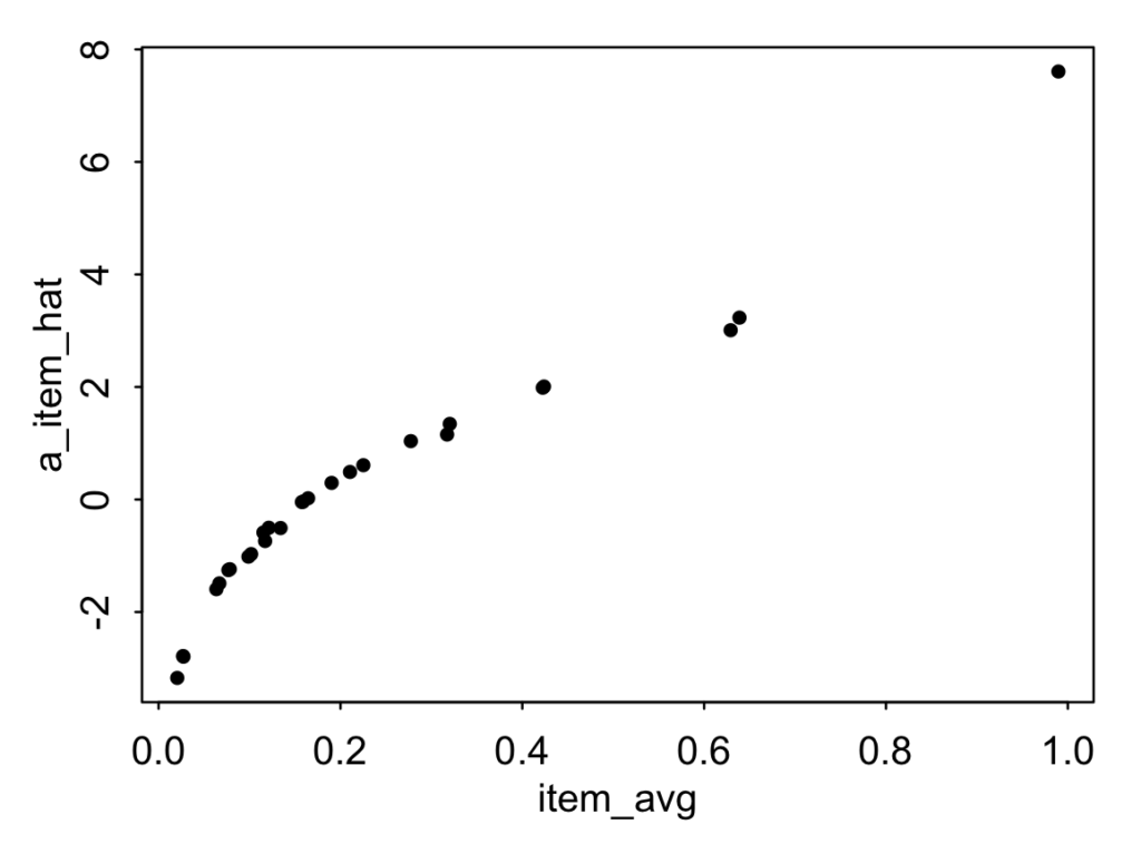
The raw rates range from 2% saying that the kite violates the rule to 99% saying that car violates the rule. Again, it's surprising to me these aren't 0% and 100% but maybe some respondents were taking the piss.

I'll re-plot labeling the points and on the logit scale:

plot(logit(item_avg), a_item_hat, type="n")
text(logit(item_avg), a_item_hat, names(a_item_hat), cex=.5)

You can't read all the items but you get the basic idea.

For the purpose of estimating these parameters we didn't really need the item-response model, but that's because the data are balanced: people were given the items randomly. In general with this sort of rating problem, it's important to fit this sort of model to account for systematic differences in who rates which items.

Just for laffs we can look at the parameter estimates and data averaged by respondents:

a_respondent_hat <- unlist(ranef(fit_lme4)$respondent)
respondent_avg <- rep(NA, J)
for (j in 1:J) {
  respondent_avg[j] <- mean(y[respondent==j])
}
plot(respondent_avg, a_respondent_hat, pch=20, cex=.4)

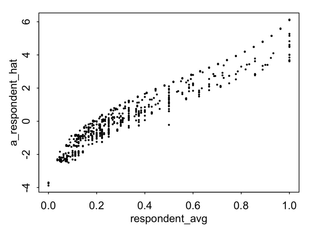
We can see a few things from the graph:
- Some number of respondents answered Yes or No to all the items. From this graph we can't see how many because of overplotting, but we can just compute sum(respondent_avg==1) and sum(respondent_avg==0) directly and find that 38 people answered Yes to all their items (that is, saying the No Vehicles in the Park rule always applies) and 10 answered only No (that is, saying that the rule never applies).
- There's quite a bit of variation in how people respond--this is something we can also see from the large value for the estimated variation of these intercepts in the fitted model.
- There's some variation in the scatterplot, which is mostly coming from variation in the number of items that people answered. The fewer items you answer, the more your intercept is partially pooled toward the mean of the distribution (zero, in this case).

3.3. Understanding the fitted model

OK, that was a real rabbit hole! Now let's return to the fitted multilevel logistic regression, fit_lme4

               coef.est coef.se
(Intercept)    -2.42     0.45  
male_name       0.07     0.03  
white_name      0.08     0.03  
n_skipped_full  0.03     0.01  

Error terms:
 Groups     Name        Std.Dev.
 respondent (Intercept) 1.92    
 item       (Intercept) 2.31    
 Residual               1.00    
---
number of obs: 51953, groups: respondent, 2409; item, 27

Going through the table from the top:
- We've already talked about the intercept.
- The coefficient for male_name is 0.07: people in this experiment are slightly more likely to say that someone with a male name is violating the rules. This is a small effect (and, yes, we can legitimately call it an "effect," as I'm pretty sure that the "treatment" of using a male or female name was assigned at random), shifting the estimated probability of "Yes, this violates the rule" from 0.24 (recall, that's the mean of y in the data) to invlogit(logit(0.24) + 0.07) = 0.253.
- The coefficient for white_name is 0.08: people in this experiment are slightly more likely to say that someone with a white name is violating the rules: again, the estimated effect is small, an estimated increased of 1.5 percentage points in the probability of a Yes response.
- People who skipped more questions are more likely to say, "Yes, this violates the rule." This effect is not so small: comparing a person who skipped 10 questions to someone who skipped none, the predicted probability of saying Yes increases from 0.24 to invlogit(logit(0.24) + 0.03*10) = 0.30.

This is kind of interesting, and it makes me think that we should also include in the model a predictor for the order in which the questions were asked. Perhaps there's a trend where, as the questions go on, people are increasingly likely to answer No.

So I'll create that new predictor:

order_of_response <- rep(NA, N)
for (j in 1:J) {
  order_of_response[respondent==j] <- 1:n_responses[j]
}
data_matrix <- data.frame(data_matrix, order_of_response)

And add it to the model:

fit_lme4 <- glmer(y ~ (1 | item) + (1 | respondent) + male_name + white_name + n_skipped_full + order_of_response, data=data, family=binomial(link="logit"))
display(fit_lme4)

Here's the result:

                  coef.est coef.se
(Intercept)       -2.59     0.45  
male_name          0.07     0.03  
white_name         0.08     0.03  
n_skipped_full     0.04     0.01  
order_of_response  0.01     0.00  

Error terms:
 Groups     Name        Std.Dev.
 respondent (Intercept) 1.92    
 item       (Intercept) 2.33    
 Residual               1.00    
---
number of obs: 51953, groups: respondent, 2409; item, 27

So, no, order of response (a predictor that varies from 1 to 27 in the data) doesn't seem to do much here. Good to know.

We conclude our understanding of the fitted model by interpreting the error variances. The distributions of respondent and item intercepts have estimated standard deviations of around 2, which is a big number on the logit scale: roughly speaking, the model estimates that about two-thirds of respondent intercepts are in the range (-1.92, 1.92), and about two-thirds of item intercepts are in the range (-2.33, 2.33). A shift of +/- 2 on the logit scale is big when you convert it to probabilities. If we start with that probability of 0.24, subtracting or adding 2 on the logit scale takes you to invlogit(logit(0.24) - 2) = 0.05 or invlogit(logit(0.24) + 2) = 0.70 on the probability scale. So, as we've already seen in the above graph, there's lots of variation across respondents and items.

4. Fitting using stan_glmer

All the above is fine. Sometimes, though, lme4 doesn't work so well. It can yield degenerate estimates for varying-intercept, varying slope models (see for example here) and, more generally, has the usual problems of point estimation that it understates uncertainty and can produce noisy estimates. So by default we prefer to use Stan, even if it's a little bit slower.

That's easy to do here using rstanarm, so first we load in that package and set it up to run parallel chains:

library("rstanarm")
options(mc.cores = parallel::detectCores())

And then we fit the model:

fit_rstanarm <- stan_glmer(y ~ (1 | item) + (1 | respondent) + male_name + white_name + n_skipped_full + order_of_response, family=binomial(link="logit"), data=data_matrix)
print(fit_rstanarm)

But in this case it takes forever. It takes so long that I hit the escape key, restarted R, and ran a minimal version:

fit_rstanarm <- stan_glmer(y ~ (1 | item) + (1 | respondent) + male_name + white_name + n_skipped_full + order_of_response, family=binomial(link="logit"), data=data_matrix, iter=200, control=list(max_treedepth=5))
print(fit_rstanarm)

There's an annoyance in the stan_glmer syntax where the number of iterations is set in one part of the function call and the treedepth is set elsewhere. This is a legacy of the rstanarm package using rstan rather than the newer interface, cmdstanr. The control options are cleaner when running Stan programs directly using cmdstanr, as we'll see below.

Anyway, to return to our main narrative, when we ran stan_glmer for 100 iterations and max treedepth of 5 and (by default) 4 chains, it's fast, but the chains do not mix well, and we get a long warning message, including this:

The largest R-hat is 4.34, indicating chains have not mixed.
Markov chains did not converge! Do not analyze results! 

Rather than chugging through thousands of iterations, I paused to think for a moment, and, from my experience fitting multilevel models, I realized the problem. It's subtle, involving both modeling and computing.

5. The funnel rears its ugly head

The problem is "the funnel," also called "the whirlpool," "the vortex," and a few other things, and it comes up with group-level variance parameters in multilevel models. David van Dyk, Zaiying Huang, John Boscardin, and I discuss the problem in this paper from 2008: the usual parameterization of the Gibbs sampler or Metropolis algorithm for such problems can get stuck when the estimated group-level variance is near zero, and the alternative, "non-centered" parameterization, can get stuck when the estimated group-level variance is near infinity. This discussion from an old version of the Stan User's Guide demonstrates the problem in a simple special case. In our 2008 paper, we recommended a redundant parameterization that works in an expanded parameter space, but this doesn't work so well with Stan, because it involves a renormalization of the parameters at each iteration.

We do not (yet) have a universal solution to the funnel problem. Here are a few options, along with their strengths and weaknesses. I'll discuss them in the context of a simple varying-intercept model with measurements i and groups j[i]:

y_i ~ normal(a_{j[i]} + X_i*beta, sigma_y), i=1,...,n
a_j ~ normal(mu, sigma_a), j=1,...,J

1. Standard parameterization as above. Works fine if sigma_a is well estimated from data and distinct from zero but runs into problems when there is posterior mass near zero, as in the 8 schools example from chapter 5 of BDA. The problem here is that in multilevel modeling you typically want sigma_a to become indistinguishable from zero: that's desirable behavior if you include high-quality group-level predictors in X.

2. Alternative parameterization:

y_i ~ normal(mu + sigma_a*xi_{j[i]} + X_i*beta, sigma_y), i=1,...,n
xi_j ~ normal(0, 1), j=1,...,J

This is mathematically the same model as above, but now it's parameterized in terms of sigma_a and xi rather than sigma_a and a = mu + sigma_a*xi. This fixes the geometry of the posterior distribution near sigma_a=0, allowing HMC (or Gibbs or Metropolis) to slide up and down the "cone" of the joint distribution rather than getting struck in the "vortex." The alternative parameterization works just fine with the 8 schools, as demonstrated in Appendix C of BDA, and other problems where there is only weak information on the group-level scale parameter sigma_a. The bad news is that it fails in the opposite scenario in which sigma_a is well estimated with a posterior distribution that is distinct from zero.

3. Redundant parameterization:

y_i ~ normal(mu + kappa*xi_{j[i]} + X_i*beta, sigma_y), i=1,...,n
xi_j ~ normal(0, tau), j=1,...,J

This model on (kappa, tau, xi) does not separately identify kappa or tau, but it does identify their product. As we discuss in our 2008 paper, you can do Gibbs or Metropolis on this larger space and just re-compute sigma_a = kappa*tau and a = mu + kappa*xi at each iteration, and it works for both the problematic examples discussed above, along with everything in between! The bad news is that if you try this redundant parameterization in Stan or other Hamiltonian Monte Carlo (HMC)-based probabilistic programming languages, it will fail because there's no joint distribution in the probability space: HMC will just drift and never converge. And you can't even run non-convergent HMC on (kappa, tau, xi) and hope to get good inferences for the generated quantities (sigma_a, a),

4. Alternate between standard and alternative parameterizations:

The redundant parameterization includes the standard and alternative parameterizations as special cases (kappa=1 and tau=1, respectively). So, instead of jointly estimating (kappa, tau, xi), you can slide back and forth between the two parameterizations, which should give you something like 50% efficiency: not as good as the optimal parameterization for your problem but not getting stuck in the bad parameterization. This approach has two challenges: first, it makes the algorithm more complicated, especially given the problems of tuning the step size and mass matrix for HMC; second, in more complicated multilevel models with more than one grouping factor (as in the example that motivated this post!), you need to do this for each batch of parameters.

5. Decide which of the standard or alternative parameterizations to use based on a preliminary analysis of the data. As we shall see, this can work in practice--you can pick one parameterization, try it, and if you have convergence problems you can switch to the other--but it's awkward. And, again, this can run into combinatorial difficulties if you have multiple grouping factors.

6. Use a zero-avoiding and infinity-avoiding prior to rule out the bad areas of the funnel. This can work, but it's not always easy: There's no generic prior that will always solve the problem, and you have to be careful not to rule out zones in parameter space that you actually want to keep in the posterior.

7. Fit using the marginal posterior mode of the group-level variance parameter. The joint mode won't work (it has a pole at (sigma_a=0, a=mu); this is a well-known problem discussed in chapter 5 of BDA and elsewhere), but you can work with the marginal mode of sigma_a. That's what lme4 does. This works fine in the example that motivated this post, but, for harder problems, marginal-mode inference can be unstable. It often yields degenerate estimates, especially when the model includes varying slopes as well as intercepts, and even when the estimated variance parameters are not on the boundary, they can be noisy. These problems can be addressed with zero-avoiding priors (see our papers from 2013 and 2014), but then that's another required step. Indeed, one reason we wrote Stan in the first place was that lme4 was giving us problems when our models started to get complicated.

8. Other approximate algorithms. ADVI and Pathfinder are already programmed in Stan, and soon we'll have nested Laplace, which is pretty similar to lme4. These options could work well; I'll have to try them out. For now I'll just have to say they're untested, and, given that they are not trying to fully explore the posterior distribution, I expect they'll have problems.

9. New HMC implementations. Bob Carpenter has been talking about a new sampler that auto-adapts in a way so that it fits the funnel just fine. Maybe this will be in Stan soon and solve all our funnel problems?

10. Some combination of the above solutions. For example: start with a stable fast algorithm such as Pathfinder, include zero-avoiding and infinity-avoiding priors as necessary, run the new adaptive HMC algorithm, also be willing to change the parameterization if it's still running slowly. This would not represent a perfectly automatic solution but could still be a reliable workflow.

11. Resolve computing problems by simplifying the model. A big challenge with the funnel is when the unexplained group-level variance is statistically indistinguishable from zero. That's what happens in the 8 schools example. One solution here is to just set the group-level scale to zero--that is, to remove that batch of parameters from the model entirely. That's equivalent to partially pooling the group estimates all the way to the fitted model: in this setting, the model is difficult to fit in part because there's no much there to be estimated, so why not simplify? In other cases, you might be uncomfortable partially pooling all the way down, so you could pin the group-level scale to some small value--for example, sigma_a=5 in the 8 schools model--which will get rid of the funnel problem. The drawback to this approach is that it requires further human intervention and also is changing the model you're fitting.

6. Fitting the model using Stan

To return to our main thread . . . we're trying to fit the model with respondent and item effects. We had problems with rstanarm so let's try using straight-up Stan which will give us more flexibility in coding.

We put our first try into a file, park_1.stan:

data {
  int<lower=0> N, J, K, L;
  array[N] int y;
  array[N] int respondent;
  array[N] int item;
  matrix[N,L] X;
}
parameters {
  vector[L] b;
  real<lower=0> sigma_respondent, sigma_item;
  vector<offset=0, multiplier=sigma_respondent>[J] a_respondent;
  vector<offset=0, multiplier=sigma_item>[K] a_item;
}
model {
  a_respondent ~ normal(0, sigma_respondent);
  a_item ~ normal(0, sigma_item);
  y ~ bernoulli_logit(X*b + a_respondent[respondent] + a_item[item]);
}

This uses the alternative parameterization, scaling the respondent and item effects in proportion to their scale parameters, so I'm pretty sure that it will fail, just as the version from rstanarm failed. But we'll check.

In R, we set up the design matrix and the data list to be sent to Stan:

X <- cbind(rep(1,N), male_name, white_name, n_skipped_full, order_of_response)
stan_data <- list(N=N, J=J, K=K, L=ncol(X), y=y, respondent=respondent, item=item, X=X)

Then we compile and run; to be on the safe side we just do 100 warmup and 100 saved iterations per chain and set max_treedepth=5:

library("cmdstanr")
park_1 <- cmdstan_model("park_1.stan")
fit_1 <- park_1$sample(data=stan_data, parallel_chains=4, iter_warmup=100, iter_sampling=100, max_treedepth=5)
print(fit_1)

Here's the (bad) result:

         variable      mean    median      sd    mad        q5       q95 rhat ess_bulk ess_tail
 lp__             -23496.85 -22783.60 1468.31 332.40 -26998.40 -22548.48 2.95        4       12
 b[1]                 -1.14     -1.14    0.18   0.23     -1.37     -0.79 2.41        5       21
 b[2]                  0.03      0.03    0.02   0.02      0.00      0.07 1.02       69      175
 b[3]                  0.03      0.03    0.03   0.03     -0.01      0.08 1.09       61      117
 b[4]                  0.03      0.02    0.00   0.00      0.02      0.03 1.19       15       48
 b[5]                 -0.01     -0.01    0.02   0.02     -0.04      0.01 2.88        4       12
 sigma_respondent      0.06      0.06    0.01   0.01      0.05      0.07 2.18        5       12
 sigma_item            1.08      1.16    0.28   0.28      0.55      1.39 3.07        4       14
 a_respondent[1]      -0.01     -0.01    0.05   0.04     -0.10      0.06 3.06        4       12
 a_respondent[2]      -0.03     -0.03    0.06   0.09     -0.12      0.05 3.94        4       12
. . .

It still has problems if you run longer. For example this is what you get if you do the default 1000 warmup plus 1000 saved iterations per chain, again setting max_treedepth=5:

         variable      mean    median     sd   mad        q5       q95 rhat ess_bulk ess_tail
 lp__             -15146.77 -15098.70 133.90 77.98 -15415.81 -15004.80 1.60        6       11
 b[1]                 -2.66     -2.71   0.34  0.24     -3.12     -1.96 1.55        8       43
 b[2]                  0.08      0.08   0.03  0.03      0.02      0.12 1.09       31      463
 b[3]                  0.07      0.07   0.03  0.04      0.02      0.13 1.24       12       76
 b[4]                  0.04      0.04   0.01  0.00      0.03      0.04 1.08      186      616
 b[5]                  0.01      0.01   0.00  0.00      0.01      0.02 1.04      444     1399
 sigma_respondent      1.92      1.94   0.07  0.06      1.80      2.01 1.54        7       12
 sigma_item            2.40      2.35   0.31  0.28      1.99      3.00 1.22       14       64
 a_respondent[1]       0.21      0.32   1.80  1.79     -2.93      3.08 1.23       12       25
 a_respondent[2]      -0.41     -0.43   0.67  0.69     -1.48      0.63 1.03      144     1040
. . .

The estimated group-level variances are big here, so it makes sense to use the standard parameterization, which is actually simpler to code in Stan. Here it is, in the file park_2.stan:

data {
  int<lower=0> N, J, K, L;
  array[N] int y;
  array[N] int respondent;
  array[N] int item;
  matrix[N,L] X;
}
parameters {
  vector[L] b;
  real<lower=0> sigma_respondent, sigma_item;
  vector[J] a_respondent;
  vector[K] a_item;
}
model {
  a_respondent ~ normal(0, sigma_respondent);
  a_item ~ normal(0, sigma_item);
  y ~ bernoulli_logit(X*b + a_respondent[respondent] + a_item[item]);
}

We'll fit this to our data, running 1000 warmup plus 1000 saved iterations per chain, max_treedepth=5:

park_2 <- cmdstan_model("park_2.stan")
fit_2 <- park_2$sample(data=stan_data, parallel_chains=4, max_treedepth=5)
print(fit_2)

It takes 100 seconds to run on my laptop, and here's what comes out:

         variable      mean    median    sd   mad        q5       q95 rhat ess_bulk ess_tail
 lp__             -16718.24 -16717.70 39.66 39.88 -16783.80 -16652.80 1.02      324      921
 b[1]                 -2.64     -2.58  0.50  0.52     -3.49     -1.82 1.43        8       13
 b[2]                  0.07      0.07  0.03  0.03      0.02      0.12 1.01      425     1137
 b[3]                  0.08      0.08  0.03  0.03      0.03      0.13 1.01      557     1135
 b[4]                  0.04      0.04  0.01  0.01      0.03      0.04 1.01      175      413
 b[5]                  0.01      0.01  0.00  0.00      0.01      0.02 1.00      863     1314
 sigma_respondent      1.96      1.96  0.04  0.04      1.89      2.03 1.04      145      280
 sigma_item            2.53      2.49  0.38  0.37      2.00      3.21 1.01      648      896
 a_respondent[1]      -0.39     -0.35  1.76  1.74     -3.41      2.49 1.01      417      956
 a_respondent[2]      -0.36     -0.32  0.70  0.66     -1.58      0.71 1.01      509      548
. . .

Not so nice! We can run it in full default setting (4 chains, 1000 warmup plus 1000 saved iterations per chain, max_treedepth=10):

fit_2 <- park_2$sample(data=stan_data, parallel_chains=4)
print(fit_2)

It now isn't too bad:

         variable      mean    median    sd   mad        q5       q95 rhat ess_bulk ess_tail
 lp__             -16714.93 -16715.20 39.87 39.88 -16780.50 -16650.59 1.00     1213     1805
 b[1]                 -2.53     -2.53  0.51  0.48     -3.40     -1.72 1.02      195      233
 b[2]                  0.07      0.07  0.03  0.03      0.02      0.12 1.00     6622     3208
 b[3]                  0.08      0.08  0.03  0.03      0.03      0.14 1.00     7494     2747
. . .

But it took 8 minutes to run. 8 minutes!

If you know what model you want to fit, and you're not worried about any problems in the data or whatever, then, sure, 8 minutes is fine, it's basically nothing. It took me a lot more than 8 minutes just to write material in this section of this post.

But if you're not sure exactly what you're planning to do, if you want to explore different models, if you want to do the usual Bayesian workflow, then you don't want to wait minutes. Not if you can avoid it.

7. A model with 3 constant terms

So what's going wrong here? We used the standard parameterization for the multilevel model, which should work better when the estimated group-level variance is large--and indeed we're now seeing better mixing for sigma_respondent and sigma_item, the group-level variance parameters--but now there's a problem with b[1], the coefficient for the constant term in the regression.

The intercept b[1] is identified in the model. The respondent effects and item effects both have distributions with mean 0. To put it another way, suppose the model were set up with:

  a_respondent ~ normal(mu_respondent, sigma_respondent);
  a_item ~ normal(mu_item, sigma_item);

Then the posterior distribution would be improper: the parameters b[1], mu_respondent, and mu_item would not be identified. To put it another way, the model would have a translation invariance, as you could add any arbitrary constants to mu_respondent and mu_item and subtract these constants from b[1] without changing the target function. By setting mu_respondent and mu_item to zero:

  a_respondent ~ normal(0, sigma_respondent);
  a_item ~ normal(0, sigma_item);

we've removed this invariance: the respondent and item effects are softly constrained toward zero. The constraint is "soft" rather than "hard" on the a_respondent and a_item parameters because the hard constraint is on the mean of their distribution; conditional on sigma_respondent and sigma_item, the respondent and item effects have informative priors centered at zero.

But . . . the soft constraint is not enough in this problem. Or, to put it more precisely, it's enough to identify the parameters but not enough to ensure smooth computation. In this model there are high posterior correlations between b[1], sum(a_respondent), and sum(a_item), and it's hard for our Hamiltonian Monte Carlo in its default settings to move efficiently in this space. Stan does some adaptation, but I think the adaptation is on the diagonal of the mass matrix so it doesn't correct for the correlations.

What to do?

I mentioned this problem to some colleagues, and they suggested using Stan's new sum_to_zero_vector type, as explained in this case study from Mitzi Morris. Here's how it works in the No Vehicles in the Park example--I put it in the file park_3.stan:

data {
  int<lower=0> N, J, K, L;
  array[N] int y;
  array[N] int respondent;
  array[N] int item;
  matrix[N,L] X;
}
parameters {
  vector[L] b;
  real<lower=0> sigma_respondent, sigma_item;
  sum_to_zero_vector[J] a_respondent;
  sum_to_zero_vector[K] a_item;
}
model {
  a_respondent ~ normal(0, sigma_respondent);
  a_item ~ normal(0, sigma_item);
  y ~ bernoulli_logit(X*b + a_respondent[respondent] + a_item[item]);
}

Here's the R code:

park_3 <- cmdstan_model("park_3.stan")
fit_3 <- park_3$sample(data=stan_data, parallel_chains=4, max_treedepth=5)
print(fit_3)

It runs in 100 seconds with this perfect mixing:

        variable      mean    median    sd   mad        q5       q95 rhat ess_bulk ess_tail
 lp__             -16714.82 -16714.70 38.92 38.99 -16779.30 -16651.30 1.00     1137     1894
 b[1]                 -2.60     -2.60  0.06  0.06     -2.70     -2.50 1.00     2237     2939
 b[2]                  0.07      0.07  0.03  0.03      0.02      0.12 1.00     7398     3227
 b[3]                  0.08      0.08  0.03  0.03      0.03      0.13 1.00     9024     2887
 b[4]                  0.04      0.04  0.01  0.01      0.03      0.05 1.00     1426     2576
 b[5]                  0.01      0.01  0.00  0.00      0.01      0.02 1.00     4123     3391
 sigma_respondent      1.95      1.95  0.04  0.04      1.89      2.02 1.00     2023     2919
 sigma_item            2.48      2.44  0.38  0.36      1.96      3.14 1.00     8438     2806
 a_respondent[1]      -0.33     -0.28  1.72  1.75     -3.20      2.47 1.00     2998     2964
 a_respondent[2]      -0.36     -0.34  0.67  0.67     -1.51      0.71 1.00     5091     2466
. . .

That's a win!

There is some awkwardness to this model: with the sum of the respondent and item effects constrained to zero, some extra mathematical effort is required when making inferences for new items and new respondents.

8. Two simulation experiments

I'm curious about a couple of things here. First, is this weak-identification thing a problem with this particular dataset or would it arise with data simulated from the model? Second, yeah yeah I get it that the correlations cause a problem with the non-sum-to-zero model, but does this also have something to do with the nonlinearity of the logit?

We can answer--or, at least, study--both these questions using simulation, first by simulating data from the fitted multilevel logistic model, second by fitting the normal rather than logit model.

First the simulation. We'll use the simulated data y_sim from Section 3.2 above and then try fitting all these models:

stan_data_sim <- stan_data
stan_data_sim$y <- y_sim
fit_1_sim <- park_1$sample(data=stan_data_sim, parallel_chains=4, max_treedepth=5)
print(fit_1_sim)
fit_2_sim <- park_2$sample(data=stan_data_sim, parallel_chains=4, max_treedepth=5)
print(fit_2_sim)
fit_3_sim <- park_3$sample(data=stan_data_sim, parallel_chains=4, max_treedepth=5)
print(fit_3_sim)

Yeah, I know my code is ugly. Feel free to clean it for your own use.

Anyway, here's what happens:
- As before, all three models took 100 seconds on my laptop.
- park_1, the model with the alternative parameterization for the group-level variance, again shows poor mixing. Not as bad as with the real data, but still unacceptable for most practical purposes.
- park_2, the model with the natural parameterization, does better but still shows poor mixing for the intercept, b[1], with an R-hat of 1.3.
- park_3, the model with the sum_to_zero constraint, has essentially perfect convergence.

So the problem was with the model, not just with the data.

Next the normal model. We could simulate data from the normal distribution, but let's just try fitting the same item-response model as before, just with a normal error term. This seems weird given that the data are binary, but we can do it. Here's the new model, park_1_normal.stan:

data {
  int<lower=0> N, J, K, L;
  vector[N] y;
  array[N] int respondent;
  array[N] int item;
  matrix[N,L] X;
}
parameters {
  vector[L] b;
  real<lower=0> sigma_respondent, sigma_item, sigma_y;
  vector[J] a_respondent;
  vector[K] a_item;
}
model {
  a_respondent ~ normal(0, sigma_respondent);
  a_item ~ normal(0, sigma_item);
  y ~ normal(X*b + a_respondent[respondent] + a_item[item], sigma_y);
}

This is the same as before, except: (a) we changed the specification of y from integer array to vector, (b) we added sigma_y as a parameter, and (c) we changed the data model from bernoulli_logit to normal.

We create park_2_normal.stan and park_3_normal.stan in the same way, then we compile and run all three:

park_normal <- list(cmdstan_model("park_1_normal.stan"),
                    cmdstan_model("park_2_normal.stan"),
                    cmdstan_model("park_3_normal.stan"))
fit_normal <- as.list(rep(NA, 3))
for (i in 1:3){
  fit_normal[[i]] <- (park_normal[[i]])$sample(data=stan_data, parallel_chains=4, max_treedepth=5)
  print(fit_normal[[i]])
}

Each one of these takes 70 seconds on my laptop--computing the gradient for the normal is a bit faster than for the logistic function, but for whatever reason it doesn't save much in compute time.

How did the computation go? Almost the same as before. Model 1 had terrible mixing, model 2 had poor mixing, but model 3 had some issues too:

        variable     mean   median    sd   mad       q5      q95 rhat ess_bulk ess_tail
 lp__             38745.21 38745.60 35.71 36.03 38685.09 38801.40 1.01      408      760
 b[1]                 0.20     0.20  0.00  0.00     0.19     0.21 1.03      114      392
 b[2]                 0.00     0.00  0.00  0.00     0.00     0.01 1.00      386     1073
 b[3]                 0.01     0.01  0.00  0.00     0.00     0.01 1.01      570      973
 b[4]                 0.00     0.00  0.00  0.00     0.00     0.00 1.09       37       68
 b[5]                 0.00     0.00  0.00  0.00     0.00     0.00 1.02      216      643
 sigma_respondent     0.19     0.19  0.00  0.00     0.18     0.19 1.01      867     1550
 sigma_item           0.23     0.23  0.03  0.03     0.18     0.29 1.04      135      207
 sigma_y              0.30     0.30  0.00  0.00     0.30     0.31 1.00     3670     2827
 a_respondent[1]     -0.04    -0.04  0.13  0.13    -0.25     0.17 1.02      124      294
. . .

This time I think the problem was with the data.

We can check with a simple simulation experiment. First we simulate data from the above-fitted model, using the posterior medians of the parameters b, sigma_respondent, sigma_item, and sigma_y, then simulating the vectors a_respondent and a_item, then simulating new data from the normal model:

library("posterior")
sims <- as_draws_rvars(fit_normal[[3]]$draws())
a_respondent_sim <- rnorm(J, 0, median(sims$sigma_respondent))
a_item_sim <- rnorm(K, 0, median(sims$sigma_item))
b_sim <- median(sims$b)
sigma_y_sim <- median(sims$sigma_y)
y_sim <- rnorm(N, a_respondent_sim[respondent] + a_item_sim[item] + X %*% b_sim, sigma_y_sim)

We then fit the three Stan models to this simulated dataset:

stan_data_sim$y <- y_sim
fit_normal_sim <- as.list(rep(NA, 3))
for (i in 1:3){
  fit_normal_sim[[i]] <- (park_normal[[i]])$sample(data=stan_data_sim, parallel_chains=4, max_treedepth=5)
  print(fit_normalsim[[i]])
}

Again, each model runs in about 70 seconds. Model 1 mixes terribly, model 2 again has problems with b[1], model 3 mixes ok, not great. Actually there's poor mixing for b[4], which is the coefficient for n_skipped. I'm really not sure why, also not sure why there's a problem for the normal model and not the binomial. That's why we do experiments--because things don't always go as expected! If you run it at default settings, mixing is fine but then it does take several minutes.

9. Summary of results

OK, we've successfully fit the model. I could talk more about summarizing the inferences for the 27 items and the 2409 respondents, and about checking the fit using posterior predictive checks, but the focus of today's post is computing.

With computing, then, where are we? What's the takeaway?

• For this example, the model fits just fine using glmer() in the lme4 package.

• lme4 computes the maximum marginal likelihood estimate of the variance parameters, averaging over the regression coefficients. Because this is a multilevel model, it doesn't work to try to maximize the joint likelihood (or find the joint posterior mode); the math on this is in chapter 5 of BDA.

• For this example, the model fails with stan_glmer() in the rstanarm package.

• For this example, the model fits fine in Stan--if you use sum_to_zero_vector.

• When the model isn't fitting well, it makes sense to run with fewer iterations and max_treedepth=5 so that you're not spinning all your cycles for fits that aren't working anyway.

• Despite the above experience for this particular dataset, we can't always recommend lme4, as it has problems when group-level variance parameters are near zero, and it has problems for varying-intercept, varying slope models.

• Surprisingly, Stan converged less well with the normal model than the binomial model.

• We hope that future developments in Stan will make this process easier:

- Nested Laplace should give us the functionality of lmer4 in a more flexible setting, not restricted to the classes of models included in that package and also allowing priors for the variance parameters

- Better adaptation should allow us to reduce the number of default iterations and also avoid the current problem where adaptation goes really slowly for the most poorly-specified models, in violation of the fail fast principle.

- Bob Carpenter told me they have a new variant of Nuts that does some sort of local adaptation which automatically works for the funnel. So then we won't need to choose between the two parameterizations.

10. Other software options

So far, we've tried lme4, rstanarm, and Stan. There are a few more options we can try.

There's INLA, which I think has pretty much the same strengths and weaknesses as lme4 for this problem, so I won't try to figure out how to use it here.

There's fast Nono, which would swallow this problem whole--but I think it only works for normal models, not logistic.

There's brms, which I think has pretty much the same strengths and weaknesses as rstanarm for this problem, so I won't try to figure out how to use it here.

And then there's variational inference. Stan has two variational methods--ADVI and Pathfinder. I'll run them in their default settings from cmdstanr. To stay focused, let's just look at model 3, the parameterization that fit well in Stan:

advi_3 <- park_3$variational(data=stan_data)
pathfinder_3 <- park_3$pathfinder(data=stan_data)

ADVI in its default setting takes 4 seconds, Pathfinder takes 70 seconds. They both yield estimates that are in the ballpark, and they both understate uncertainty compared to the model fit in full Stan, which I include below for easy comparison:

> print(advi_3)
         variable      mean    median    sd   mad        q5       q95
 lp__             -19315.46 -19312.10 59.06 60.49 -19416.52 -19222.58
 lp_approx__       -1220.23  -1219.59 35.18 35.89  -1278.46  -1161.80
 b[1]                 -2.70     -2.70  0.01  0.01     -2.72     -2.68
 b[2]                  0.06      0.06  0.03  0.02      0.02      0.10
 b[3]                  0.09      0.09  0.06  0.06     -0.01      0.19
 b[4]                  0.01      0.01  0.00  0.00      0.01      0.02
 b[5]                  0.00      0.00  0.00  0.00      0.00      0.00
 sigma_respondent      2.08      2.08  0.03  0.03      2.03      2.13
 sigma_item            2.62      2.57  0.37  0.36      2.07      3.29
 a_respondent[1]      -0.80     -0.81  0.95  0.99     -2.38      0.82
. . .
> print(pathfinder_3)
         variable      mean    median   sd  mad        q5       q95
 lp_approx__       -1250.91  -1250.91 0.00 0.00  -1250.91  -1250.91
 lp__             -18120.00 -18120.00 0.00 0.00 -18120.00 -18120.00
 b[1]                 -2.23     -2.23 0.00 0.00     -2.23     -2.23
 b[2]                  0.07      0.07 0.00 0.00      0.07      0.07
 b[3]                  0.01      0.01 0.00 0.00      0.01      0.01
 b[4]                  0.04      0.04 0.00 0.00      0.04      0.04
 b[5]                  0.01      0.01 0.00 0.00      0.01      0.01
 sigma_respondent      1.36      1.36 0.00 0.00      1.36      1.36
 sigma_item            2.13      2.13 0.00 0.00      2.13      2.13
 a_respondent[1]      -0.03     -0.03 0.00 0.00     -0.03     -0.03
. . .
> print(fit_3)
        variable      mean    median    sd   mad        q5       q95 rhat ess_bulk ess_tail
 lp__             -16714.82 -16714.70 38.92 38.99 -16779.30 -16651.30 1.00     1137     1894
 b[1]                 -2.60     -2.60  0.06  0.06     -2.70     -2.50 1.00     2237     2939
 b[2]                  0.07      0.07  0.03  0.03      0.02      0.12 1.00     7398     3227
 b[3]                  0.08      0.08  0.03  0.03      0.03      0.13 1.00     9024     2887
 b[4]                  0.04      0.04  0.01  0.01      0.03      0.05 1.00     1426     2576
 b[5]                  0.01      0.01  0.00  0.00      0.01      0.02 1.00     4123     3391
 sigma_respondent      1.95      1.95  0.04  0.04      1.89      2.02 1.00     2023     2919
 sigma_item            2.48      2.44  0.38  0.36      1.96      3.14 1.00     8438     2806
 a_respondent[1]      -0.33     -0.28  1.72  1.75     -3.20      2.47 1.00     2998     2964
. . .

Actually, Pathfinder shows no uncertainty at all, and it also returns the warning, "Pareto k value (9.2) is greater than 0.7. Importance resampling was not able to improve the approximation, which may indicate that the approximation itself is poor."

ADVI is so fast that maybe it could be good as a starting point for Stan's default NUTS algorithm.

Let's try it! First, Model 1:

advi_1 <- park_1$variational(data=stan_data)
fit_after_advi_1 <- park_1$sample(data=stan_data, init=advi_1, parallel_chains=4, max_treedepth=5)
print(fit_after_advi_1)

After the usual hundred seconds, here's what we see:

         variable      mean    median    sd   mad        q5       q95 rhat ess_bulk ess_tail
 lp__             -15074.93 -15074.55 50.84 52.11 -15158.91 -14991.80 1.02      193      436
 b[1]                 -2.54     -2.52  0.46  0.48     -3.35     -1.86 1.40        8       19
 b[2]                  0.07      0.07  0.03  0.03      0.02      0.13 1.03      335      782
 b[3]                  0.08      0.08  0.03  0.03      0.03      0.14 1.01      345      569
 b[4]                  0.04      0.04  0.01  0.01      0.03      0.04 1.04       77      138
 b[5]                  0.01      0.01  0.00  0.00      0.01      0.02 1.01      594     1121
 sigma_respondent      1.96      1.95  0.04  0.04      1.89      2.02 1.02      187      357
 sigma_item            2.49      2.41  0.38  0.34      2.01      3.24 1.07       51      107
 a_respondent[1]      -0.36     -0.26  1.71  1.77     -3.33      2.35 1.01      293      648
 a_respondent[2]      -0.31     -0.27  0.70  0.69     -1.57      0.75 1.01      388      583
. . .

It's not magic--there are still problems with mixing--but it's not bad, either. Similarly when we do with model 2. So for this problem I think that the best option is to run full Stan with max_treedepth=5 and using ADVI as a starting point. Ideally with model 3, but even with one of the poorly-mixing models we still end up with a reasonable answer. It's definitely a better option than running for 8 minutes and still not mixing.

11. Conclusion

It's not always so easy to fit multilevel models. And this model was a pretty easy one! Granted, it had non-nested groupings, but other than that it was simplicity itself: logistic regression with a few predictors and two batches of varying intercepts. For our data and model, lme4 did the job just fine--but we know that in harder problems lme4 can fail. Unfortunately, rstanarm did not work well at all--it was a problem with the parameterization used for the group-level scale parameter. Stan worked, but to avoid it taking too long, we needed a few tricks: (a) use of the right parameterization for those scale parameters, (b) the sum-to-zero constraint on the batches of varying intercepts, (c) setting max_treedepth to a level below its default of 10. Using ADVI as a starting point could make sense too.

This can be taken as a success story (we could fit the model we wanted! using full Bayes! in a reasonable amount of time!) or as a bummer (we needed to work so hard! even for this simple model!).

The next time I work on this sort of problem I'll start with lme4. Often it fails, but when it does work, it's fast, and it's a good place to start. lme4 will rarely be my final step, though, first because I'd like to more fully account for uncertainty, and second because lme4 only works on a limited class of models.

Looking at this problem from an applied perspective, we're coming into the data analysis wanting to estimate ideal points for respondents and items. We'll also want to check the fit of the model and then use it to assess some of the claims made by Dan Luu that got us thinking about this problem in the first place (see the link at the very top of this post). And we'd probably be inclined to elaborate on the model, going far beyond whatever happens to be programmed in lme4, rstanarm, and brms.

It almost makes me want to just give up! But then I remember that all this effort is still easier than the alternative of trying to cobble together a non-model-based data summary. Also the models we're fitting here have the advantage of also working for unbalanced data, which is often an issue in item-response or ideal-point estimation. Finally, doing all the above research should be helpful for me and others working on future problems.

12. How to write this up in a way to be most useful to readers?

When writing up this sort of experience, I'm always torn between making it look clean or showing all the struggles. On one hand, the struggles are important and they give a feel of our workflow. On the other hand, as a reader you could end up getting lost in all the details. I guess the right thing to do is to first present the clean version with the best solution (in this case, that would be lme4), then discuss what to do in harder problems (in this case, just jump to the Stan program that I'm calling Model 3), and only then go back and discuss the full workflow with all the guesses and experimentation.

Perhaps when writing this up more formally I'll do those steps. For now, I'll keep it as is. It already took me many hours to get this far. And I don't think this is the final version. Indeed, I'm hoping that this post will motivate Bob, Charles, and others to put in some improvements to Stan that will allow everything to run much more smoothly! But even after this particular problem gets solved using default software, there will be new problems. The workflow of computation, simulation, and experimentation will continue.

“AI Needs Specialization to Generalize”

Ameet Talwalkar is giving a talk with the above title and this abstract:

While modern AI holds great promise, the gap between its hype and practical impact remains substantial. This talk advocates for the importance of specialization to help bridge that gap–urging researchers to tailor problem formulations, modeling approaches, data collection, and evaluation methods to concrete downstream tasks. We begin by examining the limitations of existing domain-specific foundation models–for genomics, satellite imaging, and time series–that apply techniques from core AI domains such as vision and NLP with minimal specialization. We then present recent work from CMU and Datadog AI Research that advances specialized approaches across diverse tasks: solving partial differential equations, autonomously executing complex web tasks, and proactively detecting or predicting disruptions in production software systems. These efforts highlight the critical role of domain-aware design in moving beyond shiny demos and toward meaningful AI impact.

I don’t know anything about these particular application areas, but, speaking from my own experience, I agree with the title.

“Generalize” can be taken in two ways, and both of these need specialization.

The first sort of generalization is statistical: generalizing from sample to population, from treatment to control group, and from observed data to underlying constructs of interest. For these we need a mix of statistical and substantive models, with the statistical models supplying regularization (smoothness) and the substantive models setting up the generalization. For example, with MRP the statistical model is the multilevel regression and the substantive model helps us choose what variables to poststratify on, and similarly with causal and measurement models. The point is that specialization is necessary: without experience doing this in real problems, I think it would be difficult to generalize well, whether the application is pharmacology, political forecasting, or the mapping of environmental hazards.

The second sort of generalization is across problems: we develop a method in one application area and use it in another. These methods can be differential equation models, Gaussian processes, logistic regression, bootstrapping . . . also methods in experimental design, data collection, and statistical graphics. Sometimes these methods are developed on their own, Dirac-style, from first principles or as the logical consequence of other ideas, but often they arise out of particular application areas. This was the case with least-squares fitting, correlation, MRP, and all sorts of other methods–not to mention all the developments in AI that were motivated by particular applications. In that sense, we have indeed needed specialization to generalize. It is through solving domain-specific problems have we been able to create methods that are general enough to work in other domains.

You can learn a lot from a simple simulation (example of experimental design with unequal variances for treatment and control data)

We were talking about blocking in experiments in class today, and a student asked, “When should we have unequal numbers of units in the treatment and control groups?”

I replied that the simplest example is when the treatment is expensive. You could have 10,000 people in your population but only enough budget to apply the treatment to 100 people, so 99% will be in the control group. In other settings, the treatment might be disruptive, and, again, you’d only apply it to a small fraction of the available units.

But even if cost isn’t a concern, and you just want to maximize statistical efficiency, it could make sense to assign different numbers of units to the two groups.

For example, I started to say, suppose that your outcomes are much more variable under the treatment than the control. Then to minimize the basic estimate of the treatment effect—the average outcome in the treatment group, minus the average among the controls—you’ll want more treatment observations, to account for the higher variance.

But then I paused. I was struck by confusion.

There are two intuitions here, and they go in opposite directions:

(1) Treatment observations are more variable than controls. So you need more treatment measurements, so as to get a precise enough estimate for the treatment group.

(2) Treatment observations are more variable than controls. So treatment observations are crappier, and you should devote more of your budget to the high-quality control measurements.

I had a feeling that the correct reasoning was (1), not (2), but I wasn’t sure.

So how did I solve the problem?

Brute force.

Here’s the R:

n <- 100
expt_sim <- function(n, p=0.5, s_c=1, s_t=2){
  n_c <- round((1-p)*n)
  n_t <- round(p*n)
  se_dif <- sqrt(s_c^2/n_c + s_t^2/n_t)
  se_dif
}
curve(expt_sim(100, x), from=.01, to=.99,
  xlab="Proportion of data in the treatment group",
  ylab="se of estimated treatment effect",
  main="Assuming sd of measurements is\ntwice as high for treated as for controls",
  bty="l")

And here's the result:

Oh, shoot, I really don't like how the y-axis doesn't go all the way to zero. It makes the variance reduction look more dramatic than it really is. Zero is in the neighborhood, so let's invite it in:

curve(expt_sim(100, x), from=.01, to=.99,
  xlab="Proportion of data in the treatment group",
  ylab="se of estimated treatment effect",
  main="Assuming sd of measurements is\ntwice as high for treated as for controls", 
  bty="l",
  xlim=c(0, 1), ylim=c(0, 2), xaxs="i", yaxs="i")

And we can see the answer: if there's twice as much variation in the treatment group as in the control group, then you should take twice as many measurements in the treatment group. The curve is minimized at x=2/3 (which we could check without plotting anything, but the graph provides some intuition and a sanity check). Argument (1) above is correct.

On the other hand, the standard error from the optimal design isn't much lower than the simple 50/50 design, as can be seen by computing the ratio:

print(expt_sim(100, 1/2) / expt_sim(100, 2/3))

which yields 0.95.

Thus, the better design yields a 5% reduction in standard error--that is, a 10% efficiency gain. Not nothing, but not huge.

Anyway, the main point of this post is you can learn a lot from simulation. Of course in this case the problem can be solved analytically---just differentiate (s_c^2/(1-p) + s_t^2/p) with respect to p and set the derivative to zero, and you get s_c^2/(1-p)^2 - s_t^2/p^2 = 0, thus s_c^2/(1-p)^2 = s_t^2/p^2, so p/(1-p) = s_t/s_c. That's all fine, but I like the brute-force solution.

Ph.D. student position on extreme precipitation in a changing cold climate! Using Bayesian modeling and computation! At the University of Iceland!

Birgir Hrafnkelsson writes:

The Department of Mathematics at the Faculty of Physical Sciences, University of Iceland, seeks applicants to fill a PhD student position in Statistics for a project entitled: Sub-daily extreme precipitation in a changing cold climate. The project is fully funded for 3 years by the Icelandic Centre for Research.
The project involves the development of new statistical methods that make the best use of available data for predicting extreme precipitation at sub-daily scales in a changing climate, and to make predictions on extreme precipitation accessible for end-users. A statistical model for the estimation of intensity-duration-frequency curves will be set forth. The project will provide future predictions of extreme precipitation that take into account changes in climate according to established climate change scenarios.
The student will work with a consortium of experts in Bayesian statistical modeling and computation, extreme value theory, and climate science and modeling. The experts are at the University of Iceland, the Icelandic Meteorological Office, the University of Exeter, the United Kingdom Meteorological Office, Newcastle University and the King Abdullah University of Science and Technology.
For more information, contact Prof. Birgir Hrafnkelsson ([email protected]).
The application deadline is April 9, 2025.
Information on how to apply:
https://english.hi.is/vacancies

Brrrrrrrr.

Elections for the Stan Governing Body 2025

(this post is by Charles)

Calling all members of the Stan community to action!

We’re renewing the Stan Governing Body. The SGB co-organizes StanCon and related events (such as StanConnect!), works on initiatives to fund developers, and more generally helps set the directions of the project.

From the Stan forum:

We’re renewing the Stan Governing Body (SGB) with all 5 seats up for grabs. Current SGB members may still run, however they are not guaranteed to preserve their seats. As in previous years, we will use the Stan forum for nominations.

Please respond to this post to self-nominate for either a 1-year or 2-year term on the SGB before April 14th. We encourage all nominees to briefly summarize their experiences with Stan and their goals for the SGB. Feel free to add links to any content you think is relevant. And if you know someone who you think would be a good fit for the SGB please let them know and encourage them to nominate themselves.

You can find more details on the original post.


On a more personal note…

On a more personal note, I have decided to not run for a third term. Serving for two years has been an immense privilege.

It doesn’t take much reflection to realize what an integral part of my career Stan has been (and continues to be). I discovered Stan during my first job out of college at Metrum Research Group: I was contributing to the C++ library and building features which would enable applications in Pharmacometrics. My first pull request was the matrix exponential function in 2016. My first research poster was titled “Stan functions for pharmacometrics.” My first conference talk was at StanCon 2017, aka the inaugural StanCon. The project and the people working on it encouraged me—even empowered me—to pursue a PhD in Statistics, which I did at Columbia with, as my advisor, the illustrious stranger who created this blog. Throughout the years, Stan has connected me to people, both in statistics and in many applied domains.

I must recognize that, as I dove deeper into academia, I started dedicating less and less time to Stan. I remember during my first year in grad school proposing, as a final class project, adding a new feature to Stan. The prof told that me that such work was important for the scientific community but that I needed to find something that was conceptually more substantive. I was also given a clear signal that the PhD program was to train researchers, not engineers.

It’s unfortunate that incentives in academia often misalign with the goals of developing (and maintaining!) high-quality open-source software—at least in the short term. What the creators of Stan pulled off in an academic context was remarkable and unorthodox. In the end, it took an international collaboration across academia and industry to carry the project. I can’t do everyone justice, so I’ll refer you to the list of developers.

I have often felt torn between my work as a researcher and as an engineer. Sure, sometimes you can align the goals: I did leverage that final class project to build a prototype feature in Stan and wrote a research paper on it. But this anecdote strikes me more as the exception than the rule. Even after I started working at the Flatiron Institute—an institution that champions the development of scientific software and hires full-time software engineers—I only devoted so much time to Stan. My colleague Brian Ward jokes that during my almost 3 years here, he has never seen me write any C++ (and I almost haven’t). I’m embarrassed by how much time it’s taken me to write up documentation on our suite of HMM functions; I’m not very active on the Stan forum; and it is now a StanCon tradition to have someone publicly bash me for not finishing Stan’s integrated Laplace approximation (this month I hope—Steve Bronder and I are one unit test away from completing the C++ pull request. Steve has done a lot of work to create a clean user interface.)

The reality is that I’ll never get to work full time on Stan like I did before the PhD. And I suppose that’s ok. I enjoy the “conceptual” work—that is the more methodological/theoretical research that I’ve been doing, and I trust that some of it is useful to Stan users and to the broader Bayesian modeling community. I’m actually very fond of my non-Stan collaborators—if you can believe it! But the feeling of not doing enough for Stan… yeah, that’s a real thing.

Two years ago, when the announcement for the SGB election was posted, I saw an opportunity to devote more time to the Stan project in a structured manner. The SGB does a lot and I focused on bringing back StanCon. Concretely, I co-organized StanCon’23 and StanCon’24, and laid the groundwork for StanCon’26 (yes, we’re taking a one-year break). I liked working on these conferences. Sure, it’s work, but a lot of people generously contribute their time, and if the tasks are properly delegated, it all becomes very manageable. Ultimately, it’s very rewarding to see a vision brainstormed over a zoom call come to life when we all gather, say, at a pub in Oxford, and streams of colleagues we haven’t see in months, sometimes years, keep pouring in and gathering around a large table.

I also believe that StanCon is the best applied Bayesian conference out there. Period. And I think its participants benefit immensely from attending—whether by learning a lot from the tutorials or exchanging ideas with top experts. We’re a community of doers.

I hope the next batch of SGB members will tackle this opportunity with the same ambition and pride that the past bodies have displayed. And even as some of us move on, we’ll be here to insure a smooth transition and provide support where we can.

Debate about “quantum supremacy” . . . whatever that is!

Combinatorist Gil Kalai points to these papers where he and his colleagues cast doubt on claims of “quantum supremacy” by some Google researchers:

  1. Y. Rinott, T. Shoham, and G. Kalai, Statistical Aspects of the Quantum Supremacy Demonstration, Statistical Science  (2022)
  2. G. Kalai, Y. Rinott and T. Shoham, Google’s 2019 “Quantum Supremacy” Claims: Data, Documentation, & Discussion .
  3. G. Kalai, Y. Rinott and T. Shoham, Questions and Concerns About Google’s Quantum Supremacy Claim .  (see this post .)
  4. G. Kalai, Y. Rinott and T. Shoham, Random circuit sampling: Fourier expansion and statistics.

Kalai adds:

An earlier paper that I wrote : G. Kalai, The argument against quantum computers, the quantum laws of nature, and Google’s supremacy claims, discusses quantum computers, my general theory regarding quantum computers, and some aspects of the Google experiment.

I know nothing about this, but it seemed like the sort of thing that might interest some of you, so I’m sharing it.

There’s also a connection to the replication crisis, as the claim about quantum supremacy turns upon the evaluation of stochastic data.

Why not just simulate the process a billion times and find out (almost) surely?

The thing I didn’t get from the above description is: Why can’t the original researchers just run their algorithm a billion times, and then any stochastic claim would become essentially deterministic?

I asked Kalai this question and here’s his response:

Quick background: The setting of the “quantum supremacy” claims is based on a sampling task. The probability space has size M=2^n where n is the number of qubits.

Based on samples (usually of length 500,000) produced by the quantum computer (each sample is 0-1 vector of length n) the researcher concluded that the sample is “sufficiently close” to the target distribution and achieving this is something not accessible by a classical computer when n is large.

Now, to your question:

On the practical level: one of the early concerns was that the samples are not large enough for us to understand the empirical distribution. (For small values of n we overcame this difficulty and managed to show that the empirical distribution is quite different from any proposed specific model.)

So far, the researcher did not provide larger samples (and in a few replications the researchers provided smaller samples).

So the practical answer to the question “why the original researchers can’t just run their algorithm a billion times, and then any stochastic claim would become essentially deterministic?” is simply that the original researchers are not willing to do it.

On the theoretical level: my theory (the general theory about quantum computers and not the work scrutinizing specific claims) is that samples coming from quantum computers are “noise sensitive.” This means that the empirical behavior is nonstationary and even inherently unpredictable. (Probably even more than experiments on humans or animals :) )

This claim is at the heart of matters and it contradicts the clear intuition of many experts.

Interesting. This does suggest that the Google researchers don’t really believe in their result. If you believe what you have, you’ll try to replicate it as strongly as possible. Conversely, if you treat your result as a fragile flower, this suggests you don’t completely think it’s real. Or maybe you think it’s real on some sort of deep level, but you’re not convinced you have the evidence for it.

But this is just me reasoning from Kalai’s arguments. As noted above, I don’t know anything about the topic, so it would be interesting to hear from some other experts.

StanBio Connect 2025

This is Eric.

It’s hard to follow Jesus, but here we are.

Vianey Leos Barajas and I are organizing StanBio Connect 2025 conference: https://stanbio.org

StanBio is a free, one-day online conference that will take place on Friday, 30 May 2025 from 9 am to 4 pm ET. We are interested in broad applictions of Stan in biomedicine including drug discovery and development, bioinformatics, medical devices, health economics, real-world evidence, and decision-making under uncertainty. If you are developing Stan models and want to show off your work, we hope you would consider submitting an abstract by 15 April. We are planning for keynotes to be about 45 minutes and regular talks to be about 20 minutes long.

Stay tuned for the program to be released in a month or so.

We are also looking for sponsors, with the money going directly to Stan/NumFocus to help pay for the conference and to support the development of Stan. If your organization is using Stan, please consider supporting the project by sending a note to eric dot novik at nyu dot edu.

“Why don’t machine learning and large language model evaluations report uncertainty?”

Ilan Strauss and Tim O’Reilly ask:

Why don’t ML and LLM model evaluations report uncertainty? Rarely see an interval of some kind.

– Because the models are too big (LLMs)?

– Or because their ML metrics (Accuracy, recall, precision) are assumed to be sufficient for taking into account uncertainty in predictions stemming from the model’s training data, i.e. can the model generalize / predict new data points?

They continue:

LLM behavior is also inherently uncertain. The model’s responses are highly sensitive to factors like the query, hyperparameters, and context, all of which introduce variability in a model’s outputs. . . LLMs seem to be computationally deterministic in their outputs (even if practical stuff complicates this): Given the same input and conditions, the model should generate the same probabilities for the next token. The variability we see in outputs stems largely from the sampling methods applied on top of these probabilities, such as top-k sampling or temperature sampling. These techniques introduces randomness, producing different outputs for the same input. But even without this sampling layer, uncertainty should persist in LLM evaluation results because it’s impractical to test all possible model input-output combinations. . . .

Calculating and showing model uncertainty usually comes by providing an interval . . . So, why the omission by OpenAI of uncertainty from most of its model evaluations? Maybe computer scientists aren’t always familiar with common statistical practice . . . the leading AI textbook by Stuart Russell and Peter Norvig (4th edition) [has] an entire chapter on “Quantifying Uncertainty”, but devoted largely to uncertainty facing AI in the external environment. . . .

I don’t have any answer of my own to the question, “Why don’t machine learning and large language model evaluations report uncertainty?”, for the simple reason that I don’t know enough about machine learning and large language model evaluations in the first place. I imagine they do report uncertainty in some settings.

My general recommendation to people running machine learning models is to replicate using different starting points. This won’t capture all uncertainty, not even all statistical uncertainty—you can see this by considering a simple example such as linear least squares, which converges to the same solution no matter where you start it, so in that case my try-different-starting-values trick won’t get you anywhere at all—; rather, I think of this as a way to get an approximate lower bound on Monte Carlo uncertainty of your output. To get more than that, I think you need some explicit or implicit modeling of the data collection process. An explicit model goes into a likelihood function which goes into a Bayesian analysis which produces uncertainty. An implicit model could be instantiated by repeating the computation using different datasets as obtained by cross validation or bootstrapping.

What are the grand challenges in Bayesian computation?

Here’s what Anirban Bhattacharya, Antonio Linero, and Chris Oates have to say:

Grand Challenge 1: Understanding the Role of Parametrisation

Grand Challenge 2: Community Benchmarks

Grand Challenge 3: Reliable Assessment of Posterior Approximations

They also mention “software support for the full Bayesian workflow,” which I agree is super-important.

I’d also add

Scalable computing: being able to fit the models you want to fit, on large datasets

Scalable modeling: being able to build bigger models as you get more data. We can easily expand models in some directions—adding predictors in a regression, adding terms to a spline model, adding layers to a neural net, etc.—but, in other ways, model expansion can be a challenge. Even for something as simple as multilevel regression and poststratification, we can quickly get tangled in how to program up interactions.

There are many more grand challenges in Bayesian computation. Feel free to put your ideas in the comments.

P.S. Vaguely relevant here is the article by Aki and me, “What are the most important statistical ideas of the past 50 years?” Kind of amazing that we wrote that article five years ago. Time flies!