Progress in 2023, Charles edition

Following the examples of Andrew, Aki, and Jessica, and at Andrew’s request:

Published:

Unpublished:

This year, I also served on the Stan Governing Body, where my primary role was to help bring back the in-person StanCon. StanCon 2023 took place at the University of Washington in St. Louis, MO and we got the ball rolling for the 2024 edition which will be held at Oxford University in the UK.

It was also my privilege to be invited as an instructor at the Summer School on Advanced Bayesian Methods at KU Leuven, Belgium and teach a 3-day course on Stan and Torsten, as well as teach workshops at StanCon 2023 and at the University of Buffalo.

Summer School on Advanced Bayesian Methods in Belgium

(this post is by Charles)

This September, the Interuniversity Institute for Biostatistics and statistical Bioinformatics is holding its 5th Summer School on Advanced Bayesian Methods. The event is set to take place in Leuven, Belgium. From their webpage:

As before, the focus is on novel Bayesian methods relevant to the applied statistician. In the fifth edition of the summer school, the following two courses will be organized in Leuven from 11 to 15 September 2023:

The target audience of the summer school are statisticians and/or epidemiologists with a sound background in statistics, but also with a background in Bayesian methodology. In both courses, practical sessions are organized, so participants are asked to bring along their laptop with the appropriate software (to be announced) pre-installed.

I’m happy to do a three-day workshop on Stan: we’ll have ample time to dig into a lot of interesting topics and students will have a chance to do plenty of coding.

I’m also looking forward to the course on spatial modeling. I’ve worked quite a bit on the integrated Laplace approximation (notably its implementation in autodiff systems such as Stan), but I’ve never used the INLA package itself (or one of its wrappers), nor am I very familiar with applications in ecology. I expect this will be a very enriching experience.

The registration deadline is July 31st.

Scholarships for StanCon 2023

(this post is by Charles Margossian)

Applications for the StanCon scholarships are still available. As stated on the conference website:

The purpose of the StanCon scholarship is to make StanCon a more accessible and inclusive event.

Participants who require financial assistance to attend the conference may apply for a scholarship by filling out this formThe StanCon scholarship covers registration for the tutorial and the main conference, as well as local lodging. Scholarships are awarded on a need-base, and prioritize early career scientists, including students and post-docs, and members of underrepresented groups in STEM.

Applications are reviewed on a rolling basis, and scholarships are awarded based on available funds.


Scholarships are made possible by the generosity of our sponsors for the conference: the Washington University in St Louis, Metrum Research Group, and NumFocus. We have already awarded scholarships to highly qualified applicants and we’re very excited to give them the opportunity to attend the conference.

Among the current awardees, we had some well versed Stan users, and also people who are new to Stan. And this is great: the conference gathers experts and also acts as a gateway event, notably via its tutorials, which cover the basics of Stan and more advanced topics.

As a reminder, StanCon is set to take place June 20th – 23rd at the Washington University in St Louis, Missouri.


StanCon 2023: deadline for proposals extended!

…. and good news: the proposal deadline for StanCon 2023 has been extended to **April 30th**. We are mostly looking for proposals for talks, themed sessions, and posters:

We are interested in a broad range of topics relevant to the Stan community, including:

– Applications of Bayesian statistics using Stan in all domains

– Software development to support or complement the Stan ecosystem

– Methods for Bayesian modeling, relevant to a broad range of users

– Theoretical insights on common Bayesian methods and models

– Visualization techniques

– Tools for teaching Bayesian modeling.

Proposals are reviewed on a rolling basis. Several talks have already been accepted and added to the schedule, and I’m very excited about the speakers we have so far! Topics include: applications of Stan in numerous fields (healthcare, econometrics, pharmacometrics, ….), interfacing Stan with custom inference algorithms, advances in Bayesian methodology, visualisation and monitoring of MCMC while the Markov chains are running, discussions on Stan/Torsten and Turing.jl and more.

(and this does not include some of the exciting submissions we’ve recently received, although I can’t comment too much…)

There are also some wonderful tutorials lined up. I want to emphasize that a lot of the expertise the community uses to answer questions on the stan forum (https://discourse.mc-stan.org/) is taught during these tutorials.

Here’s a link to the event page https://mc-stan.org/events/stancon2023/ and as always, questions can be addressed to [email protected].

Happy weekend everyone!

StanCon 2023: call for proposals is still open!

This year, we’re bringing back StanCon in person!

StanCon is an opportunity for members of the broader Stan community to come together and discuss applications of Stan, recent developments in Bayesian modeling, and (most importantly perhaps) unsolved problems. The conference attracts field practitioners, software developers, and researchers working on methods and theory. This year’s conference will take place on June 20 – 23 at Washington University in St Louis, Missouri.

The keynote speakers are:

  • Bob Carpenter (Flatiron Institute)
  • John Kruschke (Indiana University)
  • Mariel Finucane (Mathematica Policy Research)
  • Siddhartha Chib (Washington University in St. Louis)

Proposals for talks, sessions and tutorials are due on March 31st (though it looks like we’ll be able to extend the deadline). Posters are accepted on a rolling basis. From the website:

We are interested in a broad range of topics relevant to the Stan community, including:

  • Applications of Bayesian statistics using Stan in all domains
  • Software development to support or complement the Stan ecosystem
  • Methods for Bayesian modeling, relevant to a broad range of users
  • Theoretical insights on common Bayesian methods and models
  • Visualization techniques
  • Tools for teaching Bayesian modeling

Keep in mind that StanCon brings together a diverse audience. Material which focuses on an application should introduce the problem to non-field experts; theoretical insights should be linked to problems modelers are working on, etc.

Parallelization for Markov chain Monte Carlo with heterogeneous runtimes: a case-study on ODE-based models

(this post is by Charles)

Last week, BayesComp 2023 took place in Levi, Finland. The conference covered a broad range of topics in Bayesian computation, with many high quality sessions, talks, and posters. Here’s a link to the talk abstracts. I presented two posters at the event. The first poster was on assessing the convergence of MCMC in the many-short-chains regime. I already blogged about this research (link): here’s the poster and the corresponding preprint.

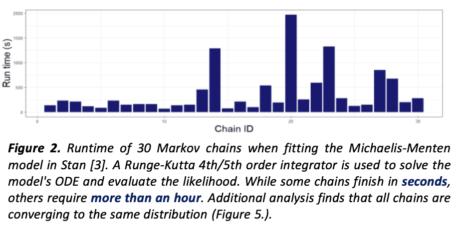
The second poster was also on the topic of running many chains in parallel but in the context of models based on ordinary differential equations (ODEs). This was the outcome of a project led by Stanislas du Ché, during his summer internship at Columbia University. We examined several pharmacometrics models, with likelihoods parameterized by the solution to an ODE. Having to solve an ODE inside a Bayesian model is challenging because the behavior of the ODE can change as the Markov chains journey across the parameter space. An ODE which is easy-to-solve at some point can be incredibly difficult somewhere else. In the past, we analyzed this issue in the illustrative planetary motion example (Gelman et al (2020), Section 11). This is the type of problem where we need to be careful about how we initialize our Markov chains and we should not rely on Stan’s defaults. Indeed, these defaults can start you in regions where your ODE is nearly impossible to solve and completely kill your computation! A popular heuristic is to draw the initial point from the prior distribution. On a related note, we need to construct priors carefully to exclude patently absurd parameter values and (hopefully) parameter values prone to frustrate our ODE solvers.

Even then—and especially if our priors are weakly informative—our Markov chains will likely journey through challenging regions. A common manifestation of this problem is that some chains lag behind because their random trajectories take them through areas that frustrate the ODE solver. Stanislas observed that this problem becomes more acute when we run many chains. Indeed, as we increase the number of chains, the probability that at least some of the chains get “stuck” increases. Then, even when running chains in parallel, the efficiency of MCMC as measured by effective sample size per second (ESS/s) eventually goes down as we add more chains because we are waiting for the slowest chain to finish!

Ok. Well, we don’t want to be punished for throwing more computation at our problem. What if we instead waited for the fastest chains to finish? This is what Stanislas studied by proposing a strategy where we stop the analysis after a certain ESS is achieved, even if some chains are still warming up. An important question is what bias does dropping chains introduce? One concern is that the fastest chains are biased because they fail to explore a region of the parameter space which contains a non-negligible amount of probability mass and where the ODE happens to be more difficult to solve. Stanislas tried to address this problem using stacking (Yao et al 2018), a strategy designed to correct for biased Markov chains. But stacking still assumes all the chains somehow “cover” the region where the probability mass concentrates and, when properly weighted, produce unbiased Monte Carlo estimators.

We may also wonder about the behavior of the slow chains. If the slow chains are close to stationarity, then by excluding them we are throwing away samples which would reduce the variance of our Monte Carlo estimators, however, it’s not worth waiting for these chains to finish if we’ve already achieved the wanted precision. What is more, as Andrew Gelman pointed out to me, slow chains can often be biased, for example if they get stuck in a pathological region during the warmup and never escape this region—as was the case in the planetary motion example. But we can’t expect this to always be the case.

In summary, I like the idea of waiting only for the fastest chains and I think understanding how to do this in a robust manner remains an open question. This work posed the problem and took steps in the right direction. There was a lot of traffic at the poster and I was pleased to see many people at the conference working on ODE-based models.

What Nested R-hat teaches us about the classical R-hat

(this post is by Charles)

My colleagues Matt Hoffman, Pavel Sountsov, Lionel Riou-Durand, Aki Vehtari, Andrew Gelman, and I released a preprint titled “Nested R-hat: assessing the convergence of Markov chain Monte Carlo when running many short chains”. This is a revision of an earlier preprint. Here’s the abstract:

The growing availability of hardware accelerators such as GPUs has generated interest in Markov chains Monte Carlo (MCMC) workflows which run a large number of chains in parallel. Each chain still needs to forget its initial state but the subsequent sampling phase can be almost arbitrarily short. To determine if the resulting short chains are reliable, we need to assess how close the Markov chains are to convergence to their stationary distribution. The R-hat statistic is a battle-tested convergence diagnostic but unfortunately can require long chains to work well. We present a nested design to overcome this challenge, and introduce tuning parameters to control the reliability, bias, and variance of convergence diagnostics.

The paper is motivated by the possibility of running many Markov chains in parallel on modern hardware, such as GPU. Increasing the number of chains allows you to reduce the variance of your Monte Carlo estimator, which is what the sampling phase is for, but not the bias, which is what the warmup phase is for (that’s the short story).  So you can trade length of the sampling phase for number of chains but you still need to achieve approximate convergence.

There’s more to be said about the many-short-chains regime but what I want to focus on is what we’ve learned about the more classic R-hat. The first step is to rewrite the condition, R-hat < 1.01, as a tolerance on the variance of the per chain Monte Carlo estimator. Intuitively, we’re running a stochastic algorithm to estimate an expectation value, which is a non-random quantity. Hence, different chains should, despite their different initialization and seed, still come to an “agreement”. This agreement is measured by the variance of the estimator produced by each chain.

Now here’s the paradox. The expected squared error of a per chain Monte Carlo estimator decomposes into a squared bias and a variance. When diagnosing convergence, we’re really interested in making sure the bias has decayed sufficiently (a common phrase is “has become negligible”, but I find it useful to think of MCMC as a biased algorithm). But, with R-hat, we’re really monitoring the variance, not the bias! So how can this be a useful diagnostic?

This paradox occurred to us when we rewrote R-hat to monitor the variance of Monte Carlo estimators constructed using groups of chains or superchains, rather than a single chain. The resulting nested R-hat decays to 1 provided we have enough chains, even if the individual chains are short (think a single iteration). But here’s the issue: regardless of wether the chains are close to convergence or not, R-hat can be made arbitrarily close to 1 by increasing the size of each superchain and thence decreasing the variance of their Monte Carlo estimator. Which goes back to my earlier point: you cannot monitor bias simply by looking at variance.

Or can you?

Here’s the twist: we now force all the chains within a superchain to start at the same point. I had this idea initially to deal with multimodal distributions. The chains within a group are no longer independent, though eventually they (hopefully) will forget about each other. In the mean time we have artificially increased the variance. Doing a standard variance decomposition:

total variance = variance of conditional expectation + expected conditional variance

Here we’re conditioning on the initial point. If the expected value of each chain no longer depends on the initialization, then the first term — variance of the conditional expectation — goes to 0. This is a measurement of “how well the chains forget their starting point”, and we call it the violation of stationarity. It is indifferent to the number of chains. The second term, on the other hand, persists even if your chains are stationary but it decays to 0 as you increase the number of chains. More generally, this persistent variance can be linked to the Effective Sample Size.

We argue that nested R-hat is a (scaled) measure of the violation of stationarity, biased by the persistent variance. How does this link to the squared bias? Well, both bias and violation decay as we warm up our chains, so one can be used as a “proxy clock” of the other. I don’t have a fully general theory for this but if you consider a Gaussian target and are willing to solve an SDE, you can show that the violation and the squared bias decay at the same rate. This is also gives us insight about how over-dispersed initializations should be (or not be) for nested R-hat to be reliable.

Now nested R-hat is a generalization of R-hat, meaning our analysis carries over! We moreover have a theory of what R-hat measures which does not assume stationarity. Part of the conceptual leap is to do an asymptotic analysis which considers an infinite number of finite (non-stationary) chains, rather than a single infinitely long (and hence stationary) chain.

Moving forward, I hope this idea of a proxy clock will help us identify cases where R-hat and its nested version are reliable, and how we might revise our MCMC processes to get more reliable diagnostics. Two examples discussed in the preprint: choice of initial variance and how to split a fixed total number of chains into superchains.

Design choices and user experience in Stan and TensorFlow Probability

(This post is by Charles, not Andrew)

I’ve been a Stan developer for a bit more than 5 years now (!!) and this summer, I interned at Google Research with the team behind TensorFlow Probability (TFP). I wanted to study a new probabilistic programming language and gain some perspective on how Stan does things. I’ll compare the two languages but rather than focus on performance, I want to talk about design and user experience. Which is fun because this aspect gets a bit lost in academic writing.

As an applied statistician, I love the Stan user experience because the focus is on modeling. Stan’s default inference is general-purpose and can be used on a very wide range of models. Other than tweaking a few tuning parameters, I usually rely on Stan’s default inference engine, which is a dynamic Hamiltonian Monte Carlo sampler. This means I can spend more time worrying about the model and whether or not it gives me the insights I seek. Being able to use “sampling” statements in the model block, i.e.

y ~ normal(theta, sigma)

is really nice because this is how I write models on paper. No graphs, no names chosen from a menu of options, no formula. For me, nothing beats writing down the generative process. Pedagogically this is a little bit confusing because any statement in Stan’s model block is not an actual sampling statement, since nothing gets sampled. Rather it’s a call to increment the log of the joint density or, in Stan’s jargon, the “target”. So maybe we should only teach the equivalent statement

target += normal_lpdf(y | theta, sigma)?

I’m not sure. Currently I teach both. I also like Stan’s coding blocks. Since a Bayesian model is specified by a joint distribution over observed variables and parameters, declaring variables in a data and parameter block further resonates with my statistical formulation of the model. There’s also another advantage: the blocks each have a different computation cost which is helpful to think about when writing computationally intensive models (see for example the discussion in this paper).

TFP acts more as a Python package than its own language. Within the same script, we’ll process the data, specify our model, run our inference, and do all the post-processing. This doesn’t have the pedagogical appeal of building blocks, nor its rigidity. Based on the tutorials I worked through, there are no pseudo-sampling statements, which means less clarity in terms of what model we’re writing down but also less confusion in terms of what computation takes place. Matt Hoffman tells me TFP has something akin to Stan’s sampling but it has less of a DSL (domain specific language) feel to it. When writing the model in TFP we can use the many functions available in Python with one super important caveat: the code needs to be differentiable, if we use gradient-based algorithms (which we probably do). With that in mind, TFP is designed to be on top of two automatic differentiation libraries: TensorFlow (surprise, surprise) and Jax. Stan has its own autodiff library so *broadly speaking* everything you write in Stan is safely differentiable. I was advised to use Jax which is pretty awesome — the documentation itself is a fascinating read. One compelling feature is that Jax supports many NumPy functions. And NumPy is great because of all the mathematical operations it offers and because it seamlessly parallelizes these operations across CPU cores. Jax takes NumPy a step further by parallelizing operations across accelerators, such as GPUs, and making a lot of these functions differentiable and therefore amiable to gradient-based inference. For those who are familiar with NumPy, this is great. For me there was a bit of a learning curve.

It’s worth pointing out that there is quite a bit of overlap between the functions Jax and Stan support but there are differences which reflect the motivating problems behind each project. Over the years, Stan’s support for ODEs has become very good and quite broad. Jax offers more specific ODE support, which works well for certain problems (e.g. Neural ODEs), less so in other cases. Note that there are pending pull requests extending Jax’s ODE support. But let’s focus on design here. Stan’s ODEs report error messages when they fail: for instance the numerical integrator reaches the maximum number of steps. Jax on the other hand reports… nothing. This is because apparently exceptions don’t exist on XLA (accelerated linear algebra, see this discussion on GitHub). Not having error messages caused me a lot of debugging grief. Overall I did find Stan did a better job issuing error and warning messages. Another example is divergent transitions: Stan automatically warns you when divergences occur. In TFP, you have to dig them out, which means you need to already know what a divergent transition is, and that may not be the case for many users.

Ok, this is where things get fun. TFP asks you to specify your inference algorithm. If you call tfp.mcmc you need to define the transition kernel of your Markov chain and usually, you should also write down an adaptive scheme. This takes a few lines of code, even if you use TFP’s built-in features. You then probably want to specify a “trace” function which records various properties of your sampler across iterations, such as whether a divergent transition occurs. This is more effort than relying on Stan’s very good defaults. But it also makes it easier to try out new transition kernels and moreover new inference algorithms! How easy is it to do this in Stan? It’s hard and this is not what Stan was designed for. That said, the underlying C++ code is open-source, well-written and well documented, and so it can be hacked. People do it. I’ve done it. And this leads to very interesting forks of Stan.

The question is: as an applied Statistician, do I resent not being able to specify my own inference algorithm in Stan? This short answer is occasionally. I’m biased because many of my scientific collaborations begin with people not being able to fit their model in Stan. Often we do eventually manage to do it by reparameterizing the model, baking more information into the priors, rewriting the ODE integrator, etc. Working out a new inference algorithm and efficiently implementing it is a bigger leap. My research does focus on the problems that frustrate our inference and for which we want to develop better methods. But this takes time. In the meantime, I believe there is a strong case to be made for an algorithm that has been stress-tested throughout the years, theoretically well-studied, and which empirically has worked for many problems.


On the other hand, as a researcher in the field of statistical algorithms, I do enjoy the modularity TFP provides and having the ability to easily try out new methods. TFP also has “experimental” features which are not fully supported but can nevertheless be tried out. I pitched the idea of including features explicitly labeled as “experimental” in Stan, as a middle-ground between making available some of the tech we’re developing and being upfront about what remains ongoing research. This gets into questions of what Stan’s mission is and how much we trust users to take heed of our warning messages. Long story short, for the time being, experimental features won’t be part of Stan’s official releases (except ADVI, which does issue a warning message).

Comparing TFP and Stan reminds me a little bit of the historical conflict between Microsoft and Apple, that is a modular approach versus end-to-end control designed to create a seamless user experience, at least on the algorithmic front. In the past I’ve approached this question by thinking about specific problems, the performance benefits of using specialized versus general techniques, and whether it makes sense to have a universal inference algorithm, or at least a universal default. But I think a big component of software development is design and user experience. How do “everyday scientists”, if you’re willing to accept this term, interact with the software? What do they want to focus on? What balance between guidance and freedom works best for a broad audience? Now when it comes to model specification, both Stan and TFP champion modularity and giving the users a large control over their model, which we could contrast to other packages out there. This too is a design choice and one we could ponder about.