We were talking about blocking in experiments in class today, and a student asked, “When should we have unequal numbers of units in the treatment and control groups?”
I replied that the simplest example is when the treatment is expensive. You could have 10,000 people in your population but only enough budget to apply the treatment to 100 people, so 99% will be in the control group. In other settings, the treatment might be disruptive, and, again, you’d only apply it to a small fraction of the available units.
But even if cost isn’t a concern, and you just want to maximize statistical efficiency, it could make sense to assign different numbers of units to the two groups.
For example, I started to say, suppose that your outcomes are much more variable under the treatment than the control. Then to minimize the basic estimate of the treatment effect—the average outcome in the treatment group, minus the average among the controls—you’ll want more treatment observations, to account for the higher variance.
But then I paused. I was struck by confusion.
There are two intuitions here, and they go in opposite directions:
(1) Treatment observations are more variable than controls. So you need more treatment measurements, so as to get a precise enough estimate for the treatment group.
(2) Treatment observations are more variable than controls. So treatment observations are crappier, and you should devote more of your budget to the high-quality control measurements.
I had a feeling that the correct reasoning was (1), not (2), but I wasn’t sure.
So how did I solve the problem?
Brute force.
Here’s the R:
n <- 100
expt_sim <- function(n, p=0.5, s_c=1, s_t=2){
  n_c <- round((1-p)*n)
  n_t <- round(p*n)
  se_dif <- sqrt(s_c^2/n_c + s_t^2/n_t)
  se_dif
}
curve(expt_sim(100, x), from=.01, to=.99,
  xlab="Proportion of data in the treatment group",
  ylab="se of estimated treatment effect",
  main="Assuming sd of measurements is\ntwice as high for treated as for controls",
  bty="l")
And here's the result:
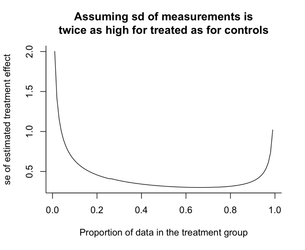
Oh, shoot, I really don't like how the y-axis doesn't go all the way to zero. It makes the variance reduction look more dramatic than it really is. Zero is in the neighborhood, so let's invite it in:
curve(expt_sim(100, x), from=.01, to=.99,
  xlab="Proportion of data in the treatment group",
  ylab="se of estimated treatment effect",
  main="Assuming sd of measurements is\ntwice as high for treated as for controls",
  bty="l",
  xlim=c(0, 1), ylim=c(0, 2), xaxs="i", yaxs="i")

And we can see the answer: if there's twice as much variation in the treatment group as in the control group, then you should take twice as many measurements in the treatment group. The curve is minimized at x=2/3 (which we could check without plotting anything, but the graph provides some intuition and a sanity check). Argument (1) above is correct.
On the other hand, the standard error from the optimal design isn't much lower than the simple 50/50 design, as can be seen by computing the ratio:
print(expt_sim(100, 1/2) / expt_sim(100, 2/3))
which yields 0.95.
Thus, the better design yields a 5% reduction in standard error--that is, a 10% efficiency gain. Not nothing, but not huge.
Anyway, the main point of this post is you can learn a lot from simulation. Of course in this case the problem can be solved analytically---just differentiate (s_c^2/(1-p) + s_t^2/p) with respect to p and set the derivative to zero, and you get s_c^2/(1-p)^2 - s_t^2/p^2 = 0, thus s_c^2/(1-p)^2 = s_t^2/p^2, so p/(1-p) = s_t/s_c. That's all fine, but I like the brute-force solution.
If instead of
“if there’s twice as much variation in the treatment group as in the control group, then you should take twice as many measurements in the treatment group. The curve is minimized at x=2/3”
does it follow that:
“if there’s n-fold as much variation in the treatment group as in the control group, then you should take n-times as many measurements in the treatment group. The curve is minimized at x=n/(n+1)”
This seems to be too simple not to have been unearthed before in clinic trials setups.
Another point: the curve which is pictured is very flat looking, indicating that getting the optimum proportion in the treatment group is not that important. Again, this seems to be too simple not to have been unearthed before in clinic trials setups.
Paul:
Yes, these results are well known. I’m not claiming originality here. The point of the post is that it’s possible to obtain and check these results directly using simulation. Indeed, it’s easier to simulate it than to go through the textbooks and literature to find the answer. Many many times I’ve seen people misread a formula and confidently get a wrong answer. I think it’s much better practice to just do the damn simulation yourself.
Guilty as charged! I’ve done this myself, more times than I care to admit. Using the wrong formula or using it incorrectly, only to discover the error through simulation which provided the right answer (even if approximate at times). Probability problems are a good example for me – correct answers elude me often, but simulation usually works.
Is there a typo in the first part of this post? I got confused by:
>“When should we have an equal number of units in the treatment and control groups?”
>I replied that the simplest example is when the treatment is expensive. You could have 10,000 people in your population but only enough budget to apply the treatment to 100 people, so 99% will be in the control group.
So shouldn’t the question be, “When should we have an UNequal number…”?
Fixed, thanks.
Cool stuff and I totally agree! Realizing the power of simulation is one of the major checkpoints on the road to quantitative fluency IMHO.
This result makes me think of something maybe less well explored. For response surface or gradient type designs where the underlying quantity increases in variance as the mean increases with our gradient (typical in many areas), should we also increase the representation of samples as we go along the gradient? Intuitively, yes, but now I’m thinking I want to simulate this :)
Wins thread (because of the last sentence of your comment).
I’m trying to come up with a scenario for which intuition #2 applies. Are you thinking more about observational studies? In a randomized experiment, the additional variance on the treatment units is presumably an effect of the treatment, rather than the measurement mechanism.
The measurement can be ‘crappy’ for at least two reasons: (1) the noise has a high variance and (2) the noise has a heavy tailed distribution. These two reasons appear similar, but they entail opposite sample size allocation. Andrew’s simulation came from (1), in which having more treatment measurements reduce estimate variance. Now let’s enter story (2), this time the control noise is still normal (0, 1), but the treatment noise is Cauchy. No matter how many samples you assign to the treatment, the treatment sample mean remains Cauchy, independent of the sample size. Of course this time you cannot evaluate the MSE of the ATE estimate because it is not finite. So let’s say we evaluate the large deviation probability Pr(ATE error > 1). What is the optimal sample size to minimize this error probability? Well, you should set the treatment samples size = 1.
Does what you say apply to a randomized experiment, in which the same measurement mechanism would be used on both arms?
Yes all the example we are discussing are RCTs. The ‘noise’ can come from both the measurement error and the population distribution, in which typically we expect a higher variation/heterogeneity in the treatment group. I think the example I gave is puzzling: the optimal treatment sample size keeps growing as the treatment group variation increases, but suddenly this optimal size drops to 1 when the variation is too big…
> The measurement can be ‘crappy’ for at least two reasons: (1) the noise has a high variance and (2) the noise has a heavy tailed distribution. These two reasons appear similar, but they entail opposite sample size allocation.
Depending on the definition of “heavy tailed”. It seems you mean (1) high finite variance and (2) infinite or undefined variance.
> Now let’s enter story (2), this time the control noise is still normal (0, 1), but the treatment noise is Cauchy.
I think that’s why Kaiser meant by “the additional variance on the treatment units is presumably an effect of the treatment, rather than the measurement mechanism”. That “noise” happens in the effect of the treatment for the individual, is not an error in the measurement on the individual.
> Of course this time you cannot evaluate the MSE of the ATE estimate because it is not finite.
The ATE itself wouldn’t exist either if the Cauchy distribution doesn’t have a mean. Let’s take the median instead.
> So let’s say we evaluate the large deviation probability Pr(ATE error > 1). What is the optimal sample size to minimize this error probability? Well, you should set the treatment samples size = 1.
Should we? Maybe if we’re going to take the mean of the outcomes, effectively discarding all the extra information provided by the additional samples. However, we can do better than that simply by taking the median of the outcomes.
I design a lot of experiments at my job and even in cases where treatment may increase the variance of outcome, I almost always default to 50/50 given the marginal gains in efficiency [as you note]. A 5% SE reduction on the margin will almost never make or break an experiment. Same logic applies for blocking subjects ahead of time on different characteristics versus just regression adjustment after the fact (or more commonly just using CUPED) in that the games are marginal.
Anon:
Relatedly, in sample surveys I usually recommend attempting simple random sampling except in cases with such high variability that there are potentially large efficiency gains. An example that has come up several times in various NYC surveys is that people want to stratify by borough. Stratification sounds like a good idea but I usually don’t recommend it, because: (a) the analysis should include all factors used in the design, so adding borough to the design implies that borough should be included in the analysis, and I usually don’t care about borough, (b) any efficiency gains will be minor, (c) there’s no need for the sample to match the population by borough anyway, (d) with rare exceptions, borough isn’t itself of interest. If you’re going to include geography in your design and analysis, I’d recommend using something like neighborhood income, so that you’re not mixing Riverdale with the South Bronx, etc.
Huh. Reading through this, intuition 1 seemed obviously right to me and intuition 2 obviously, eh, not intuitive at all. My thought process here would be: 1) you want to know about a treatment effect, which is a difference in means between C and T; 2) the quality of your estimate of this difference is, by definition, is proportional to the joint quality of the estimates of C and T (i.e. you are not primarily interested in estimating the C and T means by themselves, such that you could improve the quality of your estimate of interest by improving the quality of one mean unconditional on the quality of the estimate of the other), 3) so, if the quality of the C estimate is good and that of T is not, then obviously you allocate you resources toward improving the estimate of T. Interesting to see that you can have a completely opposite intuition.
Alex:
I can’t disagree with you: intuition 1 is correct! And it was my first guess. But once intuition 2 got into my head, I couldn’t shake it off, and it helped me to do the simulation.
I’m trying to think of a reason variance would be much higher in the treatment group and comparing the averages is an appropriate thing to do, but coming up blank.
How can this averaged information be used to benefit humankind?
Anon:
Give me a break! Not everything we do will directly “benefit humankind.” It’s indirect. Using simulation, we can better understand statistical procedures and improve our experimental design, including for studies of new treatments that might benefit humankind. This post is beneficial in that it demonstrates the simulation principle in a simple example. In the same way that a probability textbook might demonstrate certain mathematical techniques using some game of chance. There’s a long and valuable tradition of using simple examples to explain and understand scientific procedures.
Perhaps you misinterpreted. The simulation example is great. But presumably the variance is so much higher because there are important subgroups right? Eg, a drug is benefitting some and hurting others.
The original premise is that we should be averaging over all these subgroups rather than dealing with them appropriately.
In most situations where biological ‘size’ is involved, including generalizing to thinks like carbon stocks in the soil, we find that variance tends to increase with the mean. Say we do an intervention that increases crop production like N fertilization. I expect to see higher variance in that group since alleviating the N deficiency allows other limiting factors and interactions to come into play, which we may or may not be able to explicitly model very well…the usual ‘factor ceiling’ type situation. Models with unequal variances are handy here, and it’s interesting to see how this relates to design for sample size IMO.
Meinhard Kieser and his group at Heidelberg have a paper in Pharmaceutical Statistics last year investigating when unequal allocation in clinical trials is optimal for trials with binary endpoint. The savings in total sample size over equal allocation tends to be small.
In my previous job in pharma, I had a pediatrics trial where we designed the allocation as 2:1 drug to placebo because investigators told us that parents of the children would prefer the higher likelihood of being allocated drug. So in this case, the reason was non-statistical but for speed of enrollment.
> I replied that the simplest example is when the treatment is expensive. You could have 10,000 people in your population but only enough budget to apply the treatment to 100 people, so 99% will be in the control group.
I believe this is the situation that led to the use of randomisation in the 1948 MRC Streptomycin Trial (though they went for roughly equal allocation).
https://pmc.ncbi.nlm.nih.gov/articles/PMC2091872/