This blog post is by Aki with some excerpts in the end from the forthcoming Bayesian Workflow book Section 5.4 A data model is not just a “likelihood”.
It seems to be increasingly common that people say likelihood when they talk about the data model.
A Bayesian model is defined by the joint distribution of the data and parameters p(y, theta). This is usually factorized as data model p(y | theta) and prior p(theta). The product of data model and prior defines the joint distribution.
When we condition on data, p(y, theta) is only a function of theta and Bayes’ rule gives the posterior as p(theta | y) propto p(y | theta) p(theta). Here p(y | theta) as a function of theta is called likelihood (function).
I have intentionally used the common notation where p(y | theta) as a function of y is the data model and p(y | theta) as a function of theta is likelihood (function). Due to this common notation, it is even more important that we use the correct names for these.
For example, with a Bernoulli data model, the data model is discrete but the likelihood is continuous. Clearly they are completely different functions. A very long time ago, a student asked “How is it possible that combining a discrete binomial model and a continuous beta prior gives a continuous posterior?”. So it is crucial to understand that the likelihood function is not binomial but has the shape of a beta function!
We need generative models, data models, for prior checking. If you combine the likelihood and prior you get the posterior. If you combine the prior and data model, you get the prior predictive distribution!
You can’t always figure out the data model from the likelihood. The classic example is a (discrete) Poisson model for the number of events in a given time and a gamma model for the waiting time until a certain number of events. Both have gamma-shaped likelihoods, and knowing that function does not tell us what the data model is!
When, for example, in Stan you write
y ~ normal(mu, sigma);
this is read “y is distributed as normal with parameters mu and sigma”.
We can also write
target += normal_lpdf(y | mu, sigma);
and if y is data, then we are incrementing target with log-likelihood.
In simple models, the data model is easy to distinguish from the prior. But with hierarchical and missing data models there is no sharp division between parameters and data, as a model can have latent data that are not observed but are still given a generative model. For example, in the case of partially censored data, we may have observations y_obs and censored observations y_cens for which we know that they are larger than a known censoring threshold 𝑈. We can write a joint model (as this blog doesn’t allow equations, here’s a screenshot from the Bayesian Workflow book)
Here, y_cens are given the same generative data model as y_obs, and U doesn’t have a model at all. If we define the model before the data are observed, then it is not possible to say in a model like this where the data model ends and the prior begins. It depends upon which observations are censored, once the data arrive.
Another screenshot from the Bayesian Workflow book:

And yet another example:
I hope these examples illustrate why it is important to correctly use the terms data model and likelihood, and not call everything likelihood. In easy cases it is possible to understand from the context when the term likelihood is wrongly used, but if you keep using it in simple cases, you make things difficult in more elaborate cases.
We discuss data models and likelihoods much more in the forthcoming Bayesian Workflow book (expected publication date in June).
ps. A data model is also sometimes called the sampling distribution, the observation distribution, or the residual distribution; these correspond to different data structures (sampling from a population, noisy measurement of a latent process, and residuals from an additive model). We use the more general term “data model” to allow for all these scenarios.
I am afraid I do not fully understand your notation, and therefore your point. Permit me to ask a clarifying question. Am I right in thinking that the likelihood is the part of the data plugged into the equation used to calculate the posterior, and that the data model is the model that generates the data at an individual level?
In the Bernoulli case, this would mean that the data model is a function with a discrete codomain and the likelihood has a continuous codomain. Have I understood this correctly?
> Am I right in thinking that the likelihood is the part of the data plugged into the equation used to calculate the posterior
Likelihood function depends on the data
> the data model is the model that generates the data at an individual level?
We don’t necessarily know how the data is generated. The data model is model for data jointly or individually
I think de Finetti called the whole model specified before analysing the data the “prior”, i.e., not only the prior distribution over parameters is “prior”, also the parametric sampling model (and of course any hyperpriors). According to his subjectivist philosophy, all of these would formalise belief in the face of uncertainty, so it wouldn’t be correct to think that the parameter prior is subjective and the sampling model is objective, as apparently some people do. One doesn’t need to be a radical subjectivist to acknowledge that the chosen sampling model is as “prior” to the data analysis as what is usually called “prior” (and what I like to call parameter prior).
This seems quite obvious, dare say intuitive, and relates nicely to the previous post. I do hope those averse to “subjective degrees of belief” place at least a little in their “assumptions” and “knowledge”. I think I believe in what I know and at least a bit in what I assume.
We do discuss where the models and priors come from in the Bayesian Workflow book. They jointly define joint model for data and parameters, and there is no separation even it is convenient to factorize that joint model.
Hi Aki:
Very insightful post. I’m certainly guilty. But I didn’t under this line…
“I have intentionally used the common notation where p(y | theta) as a function of y is the data model and p(y | theta) as a function of theta is likelihood (function).” Is there a typo in the first use of “p(y | theta)”?
I had a similar confusion at first, but after puzzling about it, I think it is intentional and is the crux of the post. In the first case, “p(y | theta)” is used to stand for the function that defines the relative frequency with which different observations would occur (i.e., the “data model”). In the second case, “p(y | theta)” is used to stand for the computation of how likely an observation is (y) given a set of parameters, i.e., the likelihood function.
I think it helps to unfold it and give the sampling distribution and the likelihood function its own name. We all know how to evaluate p(y | theta), given values of y and of theta. We can then define two functions by what computer scientists and logicians call “binding” (e.g., with lambdas).
Given data y_obs, the likelihood function
L(theta) = p(y_obs | theta).
Here y_obs is a constant and theta is a bound variable. L(theta) is not a probability density or mass function.
Given parameters theta_true, the data generating distribution is
p_dg(y) = p(y | theta_true).
Here, theta_true is fixed and p_dg is a probability function (e.g., a probability mass function or probability density function).
Hence if we have p(y | theta) = bernoulli(y | theta), then L(theta) is a continuous function and p_dg(y) is a discrete probability mass function.
When people say that Bayes’s rule states that the posterior is proportional to the prior times the likelihood, they mean just that. Suppose p_prior(theta) is our prior density and L(theta) is our likelihood for observed data y_obs. Then
p(theta | y_obs) propto L(theta) * prior(theta).
Then we can be clear that, for example, it’s the likelihood that appears in Bayes’s rule and it’s the data generating distribution that is used for posterior predictive inference or prior predictive inference.
Bob:
We’ve been calling it the “data distribution” rather than the “sampling distribution” because data collection does not always involve sampling. Sometimes it’s called the “randomization distribution” or the “error distribution” but the data collection does not always involve randomization or error, either. And sometimes we call it the “data-generation process” but data collection does not always involve data generation at all–it can be that the data already exist and we are just sampling it! Etc.
As with the definitions of Bayesians in the earlier thread, the challenge is that a single mathematical concept is used in different application areas. There’s a tendency for people to want to pick one “true” or “correct” definition and treat it as fundamental.
I think that one reason I can often (but not always) avoid this trap is that when I was a kid I read about how Euclid’s five axioms, which can then be used to prove various theorems, can be replaced by just about any set of five theorems, which can themselves be taken as axioms and used to prove everything else. And then I remember in college taking an analysis class where we proved the Bolzano-Weierstrass theorem, and the professor remarked that in some treatments of the subject, that theorem was taken as an axiom. I can’t remember what axiom it was replacing.
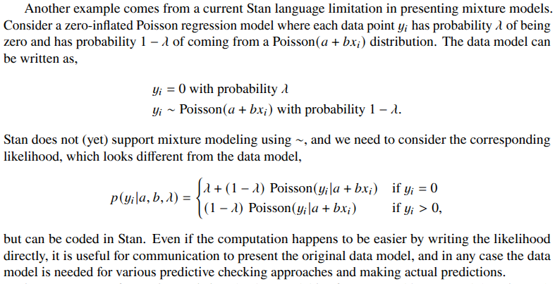
If “p(y | theta) as a function of y is the data model” when you write p(y_i|a,b, λ) how is that (as a function of y) not the data model?
y stands in for all data including individual observation y_i, future observations \tilde{y}, missing observations y_mis, censored observations, y_cens, replicated observations y_rep. This post was not meant to be extensive in the notation. We discuss this in the Bayesian Workflow book, but also in Bayesian Data Analysis, 3rd ed. theta stands in for any parameters. I did also not include data x for which we don’t necessarily have model, and thus have only partial joint distribution and condition on x. See, e.g. Section 14.1 for Bayesian justification of conditional modeling.
Maybe it was not clear but “when you write p(y_i|a,b,λ)” was a reference to the last book fragment above.
You write “we need to consider the corresponding likelihood, which looks different from the data model” and proceed to write down the probability distribution for the data p(y_i|a,b,λ) which is the data model!
Regarding the Stan language, I personally do not like the sampling statements. The target+= language better matches writing out the conditional decomposition, and it describes what is actually happening. Other than aesthetic reasons, I don’t see that the sampling statements offer anything and are probably somewhat confusing to new users…. While I always thought the sampling statement was nothing but syntactical glitter, it sounds like the above post is saying it’s supposed to represent a “data model” when in reality it’s just incrementing target with log likelihood? That just seems confusing.
Jd:
I don’t like the term “sampling statement.” Here’s what we say in the manual:
I agree that if I could go back in time to when we put together Stan, that we’d not introduced ~ and instead just used target +=.
I’m very happy that you are not able to go back in time. I love that Stan uses ~.
To clarify what Andrew says about the statements: Stan doesn’t anymore have sampling statements. The mistake was not to use ~, but to call it sampling statement, which caused people to think that the left side is sampled from the right hand side distribution, which was never the case. The correct name is distribution statement as now documented in Stan Reference Manual https://mc-stan.org/docs/reference-manual/statements.html#sampling-statements.section
Use of distribution statements is directly connected to building that joint distribution p(y, theta)
If we write the joint probability density function pi(y, theta) = pi(y | theta)pi(theta) = Bernoulli(y | theta)Beta(theta | 1, 1) via log probability density function log pi(y, theta) = log pi(y | theta) + log pi(theta) = log Bernoulli( y | theta) + log Beta(theta | 1, 1), then it seems this more directly corresponds to target+= bernoulli_lpmf(y | theta)
target += beta_lpdf(theta | 1, 1)
than the distribution syntax.
> I agree that if I could go back in time to when we put together Stan, that we’d not introduced ~ and instead just used target +=.
Interesting. I’m curious as to why they were included at the time. For historical ‘random variables’ notation styling?
Someone who worked on the language at the beginning will have to answer the question of why the notation was included, but I will say that I love love love being able to write things like:
y ~ normal(mu, sigma);
mu ~ normal(0, 10);
sigma ~ normal(0, 1);
because that maps very well to how I think about my models and if you took away the semicolons it would be exactly how I have always my models on a piece of paper when planning my code. To be able to write the model in the way that I conceive it, and then translate it so easily into Stan code, is a joy.
Unfortunately not every Stan model can be written that way, or at least that’s the case as far as I know, so I’ve had to learn the ‘target’ way of doing things too. And it’s fine. But when I can use the distribution statements I prefer to do it that way.
The sampling notation came first, then we added direct target increments later.
When I was designing the Stan language, I was working from BUGS. We needed a differentiable log density for Hamiltonian Monte Carlo and it was pretty obvious that a BUGS distribution statement like
could be compiled to C++ roughly as
Then after building that, it was also obvious that this was a general imperative language and we could add local variables and direct target increments in the object language of Stan.
We are now thinking about JAX and there we’re sticking to target +=, which is transparently coded in Python then traced by JAX. And as Aki will be happy to learn, the jax.scipy.stats.norm.logpdf function works elementwise to return the same shape as its input. JAX can then execute and sum with a parallel scan.
I’m surprised that it’s increasingly common, because my understanding is that historically Bayesians were much more tied to the likelihood principle, and generally less ecumenically-minded, than they are now.
I’d guess that what’s going is that people are just less aware of the distinction between the concepts, and the ecumenism that exists is more of “whatever works” pragmatism than a thought-through unifying perspective.