To select or not to select?

This post is by Aki

New preprint To select or not to select: predictively consistent priors instead of model selection with Anna Elisabeth Riha, Leevi Lindgren, David Kohns, Paul Bürkner and me. arXiv.2606.22850

tl;dr: Model selection is not a substitute for building good models in the first place.

Abstract: Bayesian modelling workflows often consider multiple candidate models of varying complexity. Model selection is commonly used to navigate potential trade-offs between model complexity and generalisability to new data. We study when model selection is unnecessary or can even be harmful for predictive performance in finite data regimes and find that the need for selecting simpler models can depend on prior choice. We formalise predictively consistent priors, which keep prior predictive implications stable as model complexity increases. Across examples and numerical experiments, including adding covariates in linear and logistic regression, forward variable selection, and nonlinear modelling, flexible models with predictively consistent priors typically match or outperform selected simpler models in out-of-sample predictive performance. When selection helps, it can indicate poor joint prior implications, such as excessive prior mass on implausible predictive values. Based on our findings, we propose replacing the notion of sparsity or parsimony at the level of model components with specifying priors that remain sensible in predictive space as models become more complex.

These ideas have been around, but there was no single easy paper to refer to explaining and illustrating some important aspects of model selection. Sure, model selection can reduce overfitting, but even better is to use big models and predictively consistent priors.

This is a long (76 pages) slow science paper. I had been showing variants of some plots in my talks years ago, but polishing the explanations and adding more theory took a long time. Anna, Leevi, David, and Paul all did great work on this.

Is your model converging?

This post is by Aki

I too often see people saying their model is converging or not converging. Sure, if you are doing iterative model building as part of your Bayesian workflow you could say that that iterative process eventually converges to the final model, but it seems people are actually talking about whether the inference algorithm is converging.

A Bayesian model describes a joint distribution of data and parameters. If we condition on observed data, we get the posterior distribution. We often use iterative inference algorithms to make posterior inference. If the inference algorithm doesn’t converge, the convergence problems don’t depend only on the model, but on the model, parameterisation, and the data, which together determine the geometry of the posterior. The same model and different parameterisation or data lead to different posterior geometry. For the same posterior, different iterative algorithms or algorithm choices can also lead to different convergence problems. (We have several exmples of iterative inference algorithm convergence problems in the soon to appear Bayesian workflow book)

If you want someone to help with possible inference convergence problems, it is not sufficient to tell which model you have, but you also need to tell about the parameterisation, data, and algorithm. Stop talking about models (not) converging (unless doing iterative model building) and talk about the inference algorithm (not) converging, as it is more accurate and implies dependency on the posterior and algorithm.

Looking for a postdoc to teach and develop Bayesian methods

This job ad is by Aki

I’m looking for a postdoc to help organize Bayesian Data Analysis course (200 students) and to do research on Bayesian workflow at Aalto University, Finland. Background in Bayesian topics needed. Up to five year contract possible.

Job is at Aalto University, Espoo (15min Metro ride from Helsinki center), Finland.

Starting time is flexible. There is no specific deadline, but it is better to apply soon. Apply by email (see contact information). Include CV and explanation of your skills and experience related to teaching and research.

Salary and occupational benefits are better than in academia in many other countries, and living costs are moderate (not the cheapest country but also less expensive than big cities). Finland is the world happiest country (9th time in a row)

A data model is not just a “likelihood”

This blog post is by Aki with some excerpts in the end from the forthcoming Bayesian Workflow book Section 5.4 A data model is not just a “likelihood”.

It seems to be increasingly common that people say likelihood when they talk about the data model.

A Bayesian model is defined by the joint distribution of the data and parameters p(y, theta). This is usually factorized as data model p(y | theta) and prior p(theta). The product of data model and prior defines the joint distribution.

When we condition on data, p(y, theta) is only a function of theta and Bayes’ rule gives the posterior as p(theta | y) propto p(y | theta) p(theta). Here p(y | theta) as a function of theta is called likelihood (function).

I have intentionally used the common notation where p(y | theta) as a function of y is the data model and p(y | theta) as a function of theta is likelihood (function). Due to this common notation, it is even more important that we use the correct names for these.

For example, with a Bernoulli data model, the data model is discrete but the likelihood is continuous. Clearly they are completely different functions. A very long time ago, a student asked “How is it possible that combining a discrete binomial model and a continuous beta prior gives a continuous posterior?”. So it is crucial to understand that the likelihood function is not binomial but has the shape of a beta function!

We need generative models, data models, for prior checking. If you combine the likelihood and prior you get the posterior. If you combine the prior and data model, you get the prior predictive distribution!

You can’t always figure out the data model from the likelihood. The classic example is a (discrete) Poisson model for the number of events in a given time and a gamma model for the waiting time until a certain number of events. Both have gamma-shaped likelihoods, and knowing that function does not tell us what the data model is!

When, for example, in Stan you write

y ~ normal(mu, sigma);

this is read “y is distributed as normal with parameters mu and sigma”.

We can also write

target += normal_lpdf(y | mu, sigma);

and if y is data, then we are incrementing target with log-likelihood.

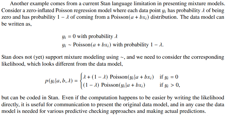
In simple models, the data model is easy to distinguish from the prior. But with hierarchical and missing data models there is no sharp division between parameters and data, as a model can have latent data that are not observed but are still given a generative model. For example, in the case of partially censored data, we may have observations y_obs and censored observations y_cens for which we know that they are larger than a known censoring threshold 𝑈. We can write a joint model (as this blog doesn’t allow equations, here’s a screenshot from the Bayesian Workflow book)

Here, y_cens are given the same generative data model as y_obs, and U doesn’t have a model at all. If we define the model before the data are observed, then it is not possible to say in a model like this where the data model ends and the prior begins. It depends upon which observations are censored, once the data arrive.

Another screenshot from the Bayesian Workflow book:


And yet another example:


I hope these examples illustrate why it is important to correctly use the terms data model and likelihood, and not call everything likelihood. In easy cases it is possible to understand from the context when the term likelihood is wrongly used, but if you keep using it in simple cases, you make things difficult in more elaborate cases.

We discuss data models and likelihoods much more in the forthcoming Bayesian Workflow book (expected publication date in June).

ps. A data model is also sometimes called the sampling distribution, the observation distribution, or the residual distribution; these correspond to different data structures (sampling from a population, noisy measurement of a latent process, and residuals from an additive model). We use the more general term “data model” to allow for all these scenarios.

Post-doc positions in Finland

This post is by Aki.

ELLIS Institute Finland is a newly established world-class research hub in AI and machine learning – and we are growing! The positions are within in one of the member universities (including Aalto University where I am).

We are now seeking postdoctoral researchers to join ELLIS Institute Finland and its wider research community. We welcome applications across all areas of machine learning, artificial intelligence, and related fields like statistics. Your research can be theoretical, applied, or span both. There are few PIs including me working also on Bayesian inference, modeling and workflow, and thus this call is great also for someone who likes these topics.

See more at the postdoc call web page.

StanCon 2026 registration and abstract submission are now open

Registration for StanCon 2026, 17-21 August, in Uppsala, Sweden, is now open! You can already register and submit abstracts for contributions. Our first keynote speaker will be announced soon.

New this StanCon: In addition to tutorials, we are introducing workshops. These are structured similarly to workshops at other conferences. We will provide three-hour rooms on the Friday of StanCon 2026 for contributor-led mini-conferences to empower the community to shape the meeting by diving deep into emerging areas and shared interests.

Submit your abstract at https://www.stancon2026.org/abstracts/

Register for StanCon 2026 at Registration – Stan Conference 2026

Deadlines

  • 28 January: Workshop and tutorial proposal deadlines; early poster acceptance deadline (for participants needing early confirmation)
  • 25 February: Oral presentation abstracts deadline
  • 27 May: Final poster submission deadline
  • 10 June: Early-bird registration deadline

Please share this announcement with anyone who might be interested!

— The Local Organising Committee
Måns Magnusson, Sara Hamis, Aki Vehtari

Effective sample size depends on the quantity

This post is by Aki.

I recently blogged about the term effective sample size and also commented “A further important point is that the effective sample size depends also on which expectation is estimated.” In the comments Visruth asked “Why does E(X^2) net a different ESS than E(X)?” and Kyurae Kim provided correct short answer. I decided to provide additional illustration

The No-U-Turn-Sampling (NUTS) variant of Hamiltonian Monte Carlo (HMC) aims to maximize the expected jump distance. The jump distance is not exactly maximized as there is randomness to keep the Markov chain reversible (which is a useful property to prove that the stationary distribution is the desired target distribution) and due to some algorithm efficiency choices. In some cases, this maximization of jump distance can lead to odd lag negative autocorrelations and higher effective sample size than the total number of draws. Let’s consider a case with theta being normally distributed. When the Markov chain is in a tail, a large jump distance will tend to take the Markov chain on the opposite side of the distribution, and if the next jump has also a large jump distance we go again to the opposite side and close to the first point. Then lag 1 and other odd lag autocorrelations are negative and lag 2 and other even lag correlations are positive. This will make effective sample size for E[theta] to be larger than the number of draws. Next it’s easiest to consider a normal distribution with mean 0 (vector of 0’s for multivariate normal) but this generalizes to non-zero means. If we now consider the absolute value of abs(theta) when we jump from tail to tail, the jump distance is likely to small and both odd and even lag autocorrelations are positive. For abs(theta) to maximize the jump distance, it would be better to jump between the tail and near mode, but NUTS is not designed to do that. theta^2 behaves as abs(theta).

We can test this with Stan and sampling from a multivariate normal. I sample from 16-dimensional unit normal, as I know that with 16 dimensions the algorithm details on how the Hamiltonian simulation is extended and U-turn decided, happen to be such that we get strong negative autocorrelations for theta.


data {
  int<lower=0> D; // number of dimensions
}
parameters {
  vector[D] theta;
}
model {
  theta ~ normal(0, 1);
}

And we run NUTS with CmdStanR

library(cmdstanr)
mod <- cmdstan_model("normal.stan")
fit <- mod$sample(data=list(D=16), refresh=0)

In the following, I examine just the first dimension of theta[1]

The autocorrelations for theta and theta^2 clearly show what I described above.

Negative autocorrelations lead to super-efficiency and the estimated ESS for theta is 10457, which is 2.6 times bigger than the total number of draws (4000). The estimated ESS for theta^2 is 1534, which is just 38% of the total number of draws! Even if we are not interested in theta^2 directly, we may be interested in sd of the posterior of theta, and computation of sd uses theta^2.

The following plot shows the ESS for the quantiles 0.05,…,0.95 (see Rank-normalization, folding, and localization: An improved Rhat for assessing convergence of MCMC for the details)

We see that if we want to report e.g. 90% posterior interval for theta, the accuracy of the interval end-points are based on about ESS of 2900. Thus, if we want to report posterior sd or posterior interval, there is not much benefit from having very high ESS for theta. In fact, as maximizing the jump distance in theta space is decreasing ESS for theta^2 and quantiles, we are wasting some computation time. However, multivariate isotropic normal is not that common posterior for most interesting models and data, and most of the time we don’t see negative autocorrelations and superefficient ESS, and thus there is no big need to change the NUTS algorithm related to this.

ESS is used to estimate Monte Carlo standard error and for any quantity of interest when MCSE is computed using, e.g., posterior package, the appropriate ESS is used. For convenience, posterior package report also Bulk-ESS and Tail-ESS which provide two summary values on the sampling efficiency in general (see the Rhat paper for the details). These are useful as quick summaries as they are scale free unlike MCSE which needs to be interpreted in the context of the scale of the quantity of interest (see more in the Digits case study).

EDIT: added 0 break for y axis

Effective sample size

This post is by Aki

Richard McElreath had a bsky post with a MCMC convergence diagnostic plot with one axis label saying “number of effective samples”. I commented that it’s wrong and misleading, and it would be better to write “effective sample size”. Frank Harrell asked elaboration. Before I had time to answer, some other people had posted just fine answers. I wanted to write a bit more but not having time to write short, I decided to write a blog post.

The problem with “number of effective samples” is that it sounds like some samples are effective and some are not, but the effectiveness is not a property of individual samples but the whole sample.

Before I continue further, I want to switch using different words. Each individual posterior draw is sample, and the collection of all posterior draws is sample. Technically this is correct, but can lead to confusion whether we refer to an individual (sample) or the group of individuals (sample). This is why I prefer to talk about individual posterior draws, and the collection of posterior draws is a posterior sample. This is also why posterior R package uses the term draw.

Every single MCMC draw has effective sample size 1, and the number of effective draws is the same as the total number of draws. However, when we use a collection of MCMC draws to estimate some expectation, the Markovian dependency makes the Monte Carlo error behave in a way that it makes sense to compare the estimation efficiency to the corresponding sample size of independent draws.

Effective sample size used to be denoted by n_eff. It might be that “number of effective samples” comes from some people reading n_eff as “number of effective”. n_eff has another problem, as n often denotes the number of observations. That’s why we recommend shortening the effective sample size as ESS. This is also what posterior package uses.

A further important point is that the effective sample size depends also on which expectation is estimated. Most commonly effective sample size has been reported for estimation of E[theta], but as the effective sample size can be very different for example for E[theta^2] it would be better to explicitly state what is estimated. By default, posterior package reports Bulk-ESS and Tail-ESS, and while neither is ESS for a simple expectation, they are more informative than just ESS.

It’s been a long time since I wrote a blog post which was not a job ad, and coincidentally also now I’m looking for postdocs who have strong background in Bayesian methods and interested to work on Bayesian cross-validation, model checking and comparison.

StanCon 2026 in Uppsala, Sweden

StanCon 2026 will take place in Uppsala, Sweden, from August 17th to August 21st, 2026.

The conference brings together researchers and practitioners passionate about Bayesian inference and probabilistic programming in one of Sweden’s most historic and vibrant university cities. Attendees will enjoy a week of conference talks, workshops, and tutorials spanning both foundational methods and real-world applications.

Stay tuned for updates! More information about registration, abstract submission, the program, and deadlines will be posted at https://www.stancon2026.org/.

The conference is sponsored by Uppsala University, The Swedish Excellence Centre for Computational Social Science at Linköping University, eSSENCE, and Beijerstiftelsen.

With kind regards from the organising committee
Måns Magnusson (Uppsala University)
Sara Hamis (Uppsala University)
Aki Vehtari (Aalto University)

Aki looking for a doctoral student to develop Bayesian workflow

I (Aki) am looking for a doctoral student with Bayesian background to work on Bayesian workflow and cross-validation (see my publication list for my recent work) at Aalto University, Finland (the world’s happiest country). You would also collaborate with Andrew and Stan and ArviZ developers. You can apply through the ELLIS PhD program (dl October 31)

loo R package 10 years!

This post is by Aki.

The loo R package has its 10 year anniversary today! Jonah Gabry made the first loo package release (v0.1.0) 10 years ago on June 26.

  • loo has been downloaded more than 4 million times from the RStudio CRAN mirror (there are more than 80 mirrors, but the RStudio mirror is likely to be one of the most popular ones)
  • R-universe counts 304 other R packages using loo
  • based on R-universe scores, loo is in top 100 among 26,819 packages

Here’s a blog post about the background, advances during the years, and a bit about the future.

Stan

When I (Aki) got involved with Stan project, there was a need for a model selection criterion that would be fast, robust, and easy to compute. I had used cross-validation (CV) a lot, but it did require some expertise to know which computational approach to use in which case, and how to diagnose the reliability. Brute-force leave-one-out cross-validation with repeated model inference is slow. Gelfand et al. (1992) had proposed importance sampling leave-one-out (LOO) CV, but 1) that estimate may have infinite variance (e.g. Peruggia, 1997), 2) due to skewed distribution the estimate would be over-optimistic with high probability, and 3) there was no good diagnostic for reliability.

DIC

Andrew had been using DIC (Spiegelhalter et al., 2002), which was simple and fast, but 1) it assumes the predictions are made using posterior mean of the parameters (and not by integrating over the posterior), 2) it’s not invariant to parameter transformations, and 3) it was known to fail for multimodal posteriors and flexible models.

WAIC

The Widely-applicable information criterion (WAIC; Watanabe, 2010) seemed promising at first, 1) being simple and fast, 2) assuming predictions using posterior predictive distribution, 3) being invariant to parameter transformations, and 4) it works with multimodal and singular posteriors. Alas, more testing of WAIC revealed it also fails with more flexible models without a warning.

Diagnostics

It was now clear that there was a pressing need for a diagnostic for the model comparison criterion computation.

I started to investigate a diagnostic for WAIC. WAIC can be presented as a truncated Taylor series approximation. In difficult cases, the higher order functional cumulant terms are not small. Can we diagnose whether MCMC estimates of higher order terms have finite variance?

Koopman et al. (2009) had proposed a diagnostic for importance sampling: 1) fit generalized Pareto distribution (GPD) to the tail of the importance ratio distribution, 2) use shape parameter k to diagnose whether the variance is finite (k <= 1/2), and 3) reject the estimate if the variance is not finite. The problem was that there was no advice what to do if the estimate is rejected and this seemed to happen a lot with WAIC and importance sampling LOO. Furthermore, finite but high variance is also problematic.

I then realized that if we assume the tail of the ratio distribution is close to a generalized Pareto distribution, and we fit the generalized Pareto distribution, we can use that as a model for the tail. To make the computation practical, this model is used to replace the raw ratios with modelled (smoothed) ratios, which are then used in further computations. In theory, modeling should reduce variability (and if the model is good, the bias can be negligible) and this was observed in practice; smoothed importance sampling LOO performed better than WAIC (or had similar performance for simple boring models).

Jonah implemented the method in loo package while we were making the experiments and writing the paper, and loo v0.1.0 was released on Github on June 26 before the papers were public.

Main papers

As theory and experiments did take a lot of pages, we decided to split the paper into “Very Good Importance Sampling” (arXived July 9, the name inspired by WAIC) and “Efficient implementation of leave-one-out cross-validation and WAIC for evaluating fitted Bayesian models” (arXived July 16). Eventually the paper names were changed to “Pareto smoothed importance sampling” (PSIS) and “Practical Bayesian model evaluation using leave-one-out cross-validation and WAIC”. The latter did get published in Statistics and Computing in less than 14 months, while the PSIS paper (final version 58 pages) took more than 9 years to get published eventually in JMLR.

While the PSIS algorithm stayed practically the same the whole time, the theoretical justifications and diagnostics did improve over the years. Dan Simpson and Yuling Yao provided help with the theory and joined as co-authors.

The PSIS estimator always has finite variance with a cost of some bias. If Pareto-k<0.7, the bias and variance are small (see details in the PSIS paper; Vehtari et al., 2024). Although 9 years felt too long time and we had a nasty case of reviewer 2, I’m happy about the improved theoretical understanding of the pre-asymptotic behaviour.

Outliers and influential observations

The loo package did gain additional practical advice on how examining the number of parameters, the effective number of parameters (p_loo), and the number of observations can provide information on whether the high Pareto-k values are likely due to a) badly misspecified model with outliers or b) well specified but flexible model.

As we get Pareto-k diagnostic for each LOO-fold, that can be used as identifying influential or problematic observations, but also to focus the additional computation only for the specific LOO-folds.

Additional computation for high Pareto-k cases

The simplest approach is to just re-run MCMC for the folds with high Pareto-k. rstanarm and brms packages know enough about the data and model, so that they can provide automated approach for this.

To speed-up computation, we developed moment matching approach (Paananen et al., 2021) that can adjust the posterior draws faster than what re-running MCMC would take, to better match the proposal and target. The needed functionality and a vignette was added to loo. brms makes it easy to use moment matching LOO with one option.

The loo package also has a vignette and support for K-fold-CV which is robust and relatively fast if, e.g. K=10.

Large data

Even though PSIS-LOO is generally fast, with big enough data it can be slow. We developed a sub-sampling LOO approach (Magnusson et al., 2019, 2022) with a vignette in the loo package. In the sub-sampling approach we use a faster but biased estimate for all LOO-folds and a slower but (almost) unbiased estimate for a subset of LOO-folds. The biggest benefits of this approach can be seen in the projpred package (github version), where PSIS-LOO given the full data search path is fast, but doing the search for each LOO-fold is slow. Using subsampling and the difference-estimator we can get more than a 10-fold speedup as demonstrated in one of the case studies.

Predictive checking

Cross-validation can be used to improve predictive checking. Posterior predictive checking can fail with flexible models as the same data are used for fitting and checking. We added useful functions to loo package to support LOO predictive checks and LOO probability integral transformation (LOO-PIT) calibration checks to bayesplot (Gabry et al., 2019; Säilynoja et al., 2022, 2025).

Beyond LOO-CV

The package is named loo as it started as an implementation of the PSIS-LOO algorithm (and we had only US and Finnish people thinking about the name). But it was natural to extend it beyond LOO.

Leave-one-group-out (LOGO) is useful if we want to predict for new groups. LOGO is challenging for importance sampling as the posterior for group specific parameters changes a lot if we leave out all the group specific observations. We can use K-fold-CV (loo vignette) or integrate out the group specific parameters (Roaches case study).

While LOO is valid for analysing the observation model in time series models, we may sometimes prefer leave-future-out cross-validation (LFO-CV), as it has smaller bias if the prediction task is in the future. The loo package has a vignette demonstrating how PSIS and occasional re-fits can be used for fast LFO-CV (Bürkner, Gabry and Vehtari, 2020).

The downside of LFO-CV is that it uses only a small part of the data for fitting the model and making predictions for the future, and thus has high variance. If the focus is model comparison, it is better to use K-fold-CV or hv-block-CV with joint log score as these have smaller variance, which leads to higher model selection efficiency for time series models (Cooper et al., 2025a).

Leaving out more than one observation and using joint log score improves the model selection efficiency also in the case of spatial models (Cooper et al., 2025b).

Often temporal and spatial models are presented as non-factorized normal (or t) models, in which case we need to use properties of multivariate normal (or t) to compute LOO (Bürkner, Gabry and Vehtari, 2020). The loo package has a vignette and brms uses this approach for non-factorized models.

Comparing models

Instead of just using point estimates of the predictive performance, we can also quantify the related uncertainty, which is especially useful when doing model comparison. From the beginning, the loo package was reporting the log score (elpd) difference and the related standard error based on the recommendation by Vehtari and Lampinen (2002). We (Sivula et al., 2025) have investigated in more detail the conditions when the standard error and related normal approximation are accurate. The normal approximation can be used to estimate probability that model B has better predictive performance than model A.

Model averaging

The LOO computed log score (elpd_loo) has a connection to information criteria (see, e.g. Vehtari and Ojanen, 2012). Inspired by information criteria based model weights and stacking, we developed Bayesian stacking (Yao et al., 2018), which is also implemented in the loo package. Furthermore, we extended Bayesian stacking to Bayesian hierarchical stacking (Yao et al., 2022a) and stacking for non-mixing computations (Yao et al., 2022b). There is a loo package vignette for stacking.

Other scores and metrics

The loo package supports also (S)CRPS, MAE, RMSE, MSE, ACC, and BACC, although not as nicely as log score (see below for future plans).

ArviZ

loo is an R package, but PyStan and PyMC users needed fast cross-validation, too. The Python and Julia ArviZ libraries were subsequently developed to include most of the methods that are in the loo R package,

Future

Because PSIS is useful in many other cases beyond just LOO, PSIS functionality has now been implemented in the posterior package, so that packages that would like to use just the Pareto smoothing and diagnostics do not need to depend on the loo package. We’re also in the progress of changing loo to use more of these functions from posterior.

We’re also refactoring loo to improve modularity and usability (as part of Google Summer of Code) focusing on:

  • easier use of different scores and metrics (e.g. RMSE, R^2, CRPS)
  • easier use of different cross-validation variants
  • easier use of joint log score
  • more diagnostic information provided to the user, e.g. for the uncertainty normal approximation

The ArviZ team is also working to update ArviZ.

CV-FAQ

The loo package users have been asking many questions, and eventually I wrote CV-FAQ answering the most frequently asked questions (and setting straight some common misconceptions).

Thanks

Very big thanks to Jonah Gabry for writing the loo package (see also other contributors) and to the ArviZ team for implementing the methods in Python and Julia! All the methods developed in the papers would not be widely used without these packages (The Practical LOO-CV paper has been cited more than 5900 times). While the methods in the papers made certain things possible, it is the software that makes using the methods easy!

Better priors for AR, ARX, LTX, DR, MA, ARMA, and VAR models

We arXived last year a paper The ARR2 prior: flexible predictive prior definition for Bayesian auto-regressions” by David Kohns, Noa Kallionen, Yann McLatchie, and me (Aki). Last week, we uploaded a revised version.

The idea of the paper is to have a prior that is predictively consistent, that is, if we add more terms (e.g., lags and covariates) to the model, the prior predictive distribution should not change substantially. This can be done by setting the prior on R-squared and using variance decomposition inspired by R2D2 prior. Using such priors allows using big models without fear of overfitting, there is no need to try to select the number of lags, and the information from the data is more efficiently used. If needed, a smaller model can be selected afterward considering the model selection as decision problem given the big model (see, e.g. Using reference models in variable selection and Advances in projection predictive inference).

The first version included the derivations for AR, ARX, LTX, and DR models. The revision adds results about implied priors on characteristic roots and partial autocorrelations, case study with quasi-cyclical behavior, and extensions to MA, ARMA, ARDL, and VAR models. The paper and associated git repo include Stan code.

9 AI/ML/comp.stat./CS professor positions at Aalto University, Finland

This is big!

Aalto University has total of 5 AI/ML/comp.stat. (note that Bayesian statistics is also considered to be AI by European Union) professor positions at different departments including our CS department:

  • Assistant Professor in Computer Science (Artificial Intelligence / Machine Learning)
  • Assistant Professor in Information and Service Management (AI Business Applications)
  • Assistant/Associate/Full Professor in Electrical Engineering (Intelligent Systems)
  • Assistant Professor in Machine Learning in Materials Science
  • Assistant Professor in Machine Learning in Chemical Processes

This is part of a big joint call with total of AI/ML 25 open professor positions in several Finnish universities in connection with the new ELLIS institute Finland! See more information and how to apply at https://www.ellisinstitute.fi/PI-recruit (deadline March 9th).

In addition, our CS department at Aalto University has 4 other CS assistant professor positions

  • Computer Architecture and Programming Languages (deadline 16 March)
  • Human-Computer Interaction (deadline 23 March)
  • Software Engineering (deadline 9 March)
  • Systems Security (deadline 9 March)

See more information and how to apply at https://www.aalto.fi/en/department-of-computer-science/assistant-professor-positions

Posterior SBC: Simulation-Based Calibration Checking Conditional on Data

If you know simulation based calibration checking (SBC), you will enjoy our new paper Posterior SBC: Simulation-Based Calibration Checking Conditional on Data with Teemu Säilynoja, Marvin Schmitt, Paul Bürkner, and Aki Vehtari

The original SBC checks whether the inference works for all possible data sets generated using the model and parameter draws from the prior. Priors are usually wider than posteriors and may contain regions where the computation fails.

For example, for hierarchical models, MCMC can have problems either with centered or non-centered parameterization depending on the data. Given one of the parameterizations, prior SBC observes both failing and non-failing inference. Posterior SBC focuses on the posterior conditional on the data, and can assess which parameterization works better for that specific data.

We illustrate with a hierarchical normal and a Lotka-Volterra models using MCMC, and a drift diffusion model using amortized Bayesian inference. Posterior SBC is specifically useful for amortized inference, as the repeated inference has negligible cost.

Postdoc, doctoral student, and summer intern positions, Bayesian methods, Aalto

Postdoc and doctoral student positions in developing Bayesian methods at Aalto University, Finland! This job post is by Aki (maybe someday I write an actual blog post).

The positions are funded by Finnish Center for Artificial Intelligence FCAI and there are many other topics, but if you specify me as the preferred supervisor then it’s going to be Bayesian methods, workflow, cross-validation, and diagnostics. See my video on Bayesian workflow, Bayesian workflow paper, my publication list, and my talk list, for more about what I’m working on.

There are also plenty of other topics and supervisors in

  1. Reinforcement learning
  2. Probabilistic methods
  3. Simulation-based inference
  4. Privacy-preserving machine learning
  5. Collaborative AI and human modeling
  6. Machine learning for science

Join us, and learn why Finland has been ranked the happiest country in the world for seven years in row!

See how to apply at fcai.fi/winter-2025-researcher-positions-in-ai-and-machine-learning

I might also hire one summer intern (BSc or MSc level) to work on the same topics. Applications through Aalto Science Institute call

Progress in 2024 (Aki)

Here’s my 2024 progress report. There are 5 publications common with Andrew in 2024.

Active Statistics book is the biggest in size, but personally getting the Pareto smoothed importance sampling paper published after 9 years from the first submission was a big event, too. I think I only blogged 2023 progress report and job ads (I sometimes have blog post ideas, but as I’m a slow writer, it’s difficult to find time to turn them to actual posts). I’m very happy with the progress in 2024, but also excited on what we are going to get done in 2025!

Book

Papers published or accepted for publication in 2024

  • Yann McLatchie, Sölvi Rögnvaldsson, Frank Weber, and Aki Vehtari (2025). Advances in projection predictive inference. Statistical Science, accepted for publication. arXiv preprint arXiv:2306.15581. Software: projpred, kulprit.

  • Christopher Tosh, Philip Greengard, Ben Goodrich, Andrew Gelman, Aki Vehtari, and Daniel Hsu (2025). The piranha problem: Large effects swimming in a small pond. Notices of the American Mathematical Society, 72(1):15-25. arXiv preprint arXiv:2105.13445.

  • Kunal Ghosh, Milica Todorović, Aki Vehtari, and Patrick Rinke (2025). Active learning of molecular data for task-specific objectives. The Journal of Chemical Physics, doi:10.1063/5.0229834.

  • Charles C. Margossian, Matthew D. Hoffman, Pavel Sountsov, Lionel Riou-Durand, Aki Vehtari, and Andrew Gelman (2024). Nested Rhat: Assessing the convergence of Markov chain Monte Carlo when running many short chains. Bayesian Analysis, doi:10.1214/24-BA1453.Software: posterior.

  • Yann McLatchie and Aki Vehtari (2024). Efficient estimation and correction of selection-induced bias with order statistics. Statistics and Computing, 34(132). doi:10.1007/s11222-024-10442-4.

  • Frank Weber, Änne Glass, and Aki Vehtari (2024). Projection predictive variable selection for discrete response families with finite support. Computational Statistics, doi:10.1007/s00180-024-01506-0. Software projpred.

  • Aki Vehtari, Daniel Simpson, Andrew Gelman, Yuling Yao, and Jonah Gabry (2024). Pareto smoothed importance sampling. Journal of Machine Learning Research, 25(72):1-58. Online. Software: loo, posterior, ArviZ

  • Manushi Welandawe, Michael Riis Andersen, Aki Vehtari, and Jonathan H. Huggins (2024). A framework for improving the reliability of black-box variational inference. Journal of Machine Learning Research, 25(219):1-71. Online.

  • Noa Kallioinen, Topi Paananen, Paul-Christian Bürkner, and Aki Vehtari (2024). Detecting and diagnosing prior and likelihood sensitivity with power-scaling. Statistics and Computing, 34(57). Online.
    Supplementary code.
    Software: priorsense

  • Erik Štrumbelj, Alexandre Bouchard-Côté, Jukka Corander, Andrew Gelman, Håvard Rue, Lawrence Murray, Henri Pesonen, Martyn Plummer, and Aki Vehtari (2024). Past, present, and future of software for Bayesian inference. Statistical Science, 39(1):46-61. Online.

  • Alex Cooper, Dan Simpson, Lauren Kennedy, Catherine Forbes, and Aki Vehtari (2024). Cross-validatory model selection for Bayesian autoregressions with exogenous regressors. Bayesian Analysis, doi:10.1214/23-BA1409.

  • Marta Kołczyńska, Paul-Christian Bürkner, Lauren Kennedy, and Aki Vehtari (2024). Trust in state institutions in Europe, 1989–2019. Survey Research Methods, 18(1). doi:10.18148/srm/2024.v18i1.8119.

  • Alex Cooper, Aki Vehtari, Catherine Forbes, Lauren Kennedy, and Dan Simpson (2024). Bayesian cross-validation by parallel Markov chain Monte Carlo. Statistics and Computing, 34:119. doi:10.1007/s11222-024-10404-w.

  • Ryoko Noda, Michael Francis Mechenich, Juha Saarinen, Aki Vehtari, Indrė Žliobaitė (2024). Predicting habitat suitability for Asian elephants in non-analog ecosystems with Bayesian models. Ecological Informatics, 82:102658. doi:10.1016/j.ecoinf.2024.102658.

  • Petrus Mikkola, Osvaldo A. Martin, Suyog Chandramouli, Marcelo Hartmann, Oriol Abril Pla, Owen Thomas, Henri Pesonen, Jukka Corander, Aki Vehtari, Samuel Kaski, Paul-Christian Bürkner, Arto Klami (2024). Prior knowledge elicitation: The past, present, and future. Bayesian Analysis, 19(49):1129-1161. doi:10.1214/23-BA1381.

arXived in 2024

  • Marvin Schmitt, Chengkun Li, Aki Vehtari, Luigi Acerbi, Paul-Christian Bürkner, and Stefan T. Radev (2024). Amortized Bayesian Workflow (Extended Abstract). arXiv preprint arXiv:2409.04332.

  • Måns Magnusson, Jakob Torgander, Paul-Christian Bürkner, Lu Zhang, Bob Carpenter, and Aki Vehtari (2024). posteriordb: Testing, benchmarking and developing Bayesian inference algorithms. arXiv preprint arXiv:2407.04967. Database and software: posteriordb

  • David Kohns, Noa Kallionen, Yann McLatchie, and Aki Vehtari (2024). The ARR2 prior: flexible predictive prior definition for Bayesian auto-regressions. arXiv preprint arXiv:2405.19920.

  • Anna Elisabeth Riha, Nikolas Siccha, Antti Oulasvirta, and Aki Vehtari (2024). Supporting Bayesian modelling workflows with iterative filtering for multiverse analysis. arXiv preprint arXiv:2404.01688.

  • Guangzhao Cheng, Aki Vehtari, and Lu Cheng (2024). Raw signal segmentation for estimating RNA modifications and structures from Nanopore direct RNA sequencing data. bioRxiv preprint.

Software

Case studies

  • Aki Vehtari (2024). Nabiximols. Model checking and comparison, comparison of continuous and discrete models, LOO-PIT checking, calibration plots, prior sensitivity analysis, model refinement, treatment effect, effect of model mis-specification.

  • Aki Vehtari (2024). Birthdays. Workflow example for iterative building of a time series model. In 2024, added demonstration of Pathfinder for quick initial results and MCMC initialization.

FAQ

Video

Doctoral student positions in Bayesian workflow at Aalto, Finland

Apply for fully funded doctoral student position to work with me (Aki) on Bayesian workflow, model selection, inference, and diagnostics!

Apply through a joint call fcai.fi/doctoral-program and choose me as the supervisor, and tell in the motivation letter why you want to work with me. DL Sep 9.

You can also ask me more about possible research topics and information how it is like to do doctoral studies at Aalto and in the Bayesian workflow group.

Research would include collaboration with Andrew, Richard McElreath, Paul Bürkner and Stan development team, and potential research visits with them.

(There are also many other topics and professors to choose from in AI, machine learning and probabilistic modeling…)

Supporting Bayesian modelling workflows with iterative filtering for multiverse analysis

There is a new paper in arXiv: “Supporting Bayesian modelling workflows with iterative filtering for multiverse analysis” by Anna Elisabeth Riha, Nikolas Siccha, Antti Oulasvirta, and Aki Vehtari.

Anna writes

An essential component of Bayesian workflows is the iteration within and across models with the goal of validating and improving the models. Workflows make the required and optional steps in model development explicit, but also require the modeller to entertain different candidate models and keep track of the dynamic set of considered models.

By acknowledging the existence of multiple candidate models (universes) for any data analysis task, multiverse analysis provides an approach for transparent and parallel investigation of various models (a multiverse) that makes considered models and their underlying modelling choices explicit and accessible. While this is great news for the task of tracking considered models and their implied conclusions, more exploration can introduce more work for the modeller since not all considered models will be suitable for the problem at hand. With more models, more time needs to be spent with evaluation and comparison to decide which models are the more promising candidates for a given modelling task and context.

To make joint evaluation easier and reduce the amount of models in a meaningful way, we propose to filter out models with largely inferior predictive abilities and check computation and reliability of obtained estimates and, if needed, adjust models or computation in a loop of changing and checking. Ultimately, we evaluate predictive abilities again to ensure a filtered set of models that contains only the models that are sufficiently able to provide accurate predictions. Just like we filter out coffee grains in a coffee filter, our suggested approach sets out to remove largely inferior candidates from an initial multiverse and leaves us with a consumable brew of filtered models that is easier to evaluate and usable for further analyses. Our suggested approach can reduce a given set of candidate models towards smaller sets of models of higher quality, given that our filtering criteria reflect characteristics of the models that we care about.

Fully funded doctoral student positions in Finland

There is a new government funded Finnish Doctoral Program in AI. Research topics include Bayesian inference, modeling and workflows as part of fundamental AI. There is a big joint call, where you can choose the supervisor you want to work with. I (Aki) am also one of the supervisors. Come work with me or share the news! The first call deadline is April 2, and the second call deadline in fall 2024. See how to apply at https://fcai.fi/doctoral-program, and more about my research at my web page.

Bayesian Analysis with Python

Osvaldo Martin writes:

The third edition of Bayesian Analysis with Python serves as an introduction to the basic concepts of applied Bayesian modeling. It adopts a hands-on approach, guiding you through the process of building, exploring and expanding models using PyMC and ArviZ. The field of probabilistic programming is in a different place today than it was when the first edition was devised in the middle of the last decade. The journey from its first publication to this current edition mirrors the evolution of Bayesian modeling itself – a path marked by significant advancements, growing community involvement, and an increasing presence in both academia and industry. Consequently, this updated edition also includes coverage of additional topics and libraries such as Bambi, for flexible and easy hierarchical linear modeling, PyMC-BART, for flexible non-parametric regression; PreliZ, for prior elicitation; and Kulprit, for variable selection.

Whether you’re a student, data scientist, researcher, or developer aiming to initiate Bayesian data analysis and delve into probabilistic programming, this book provides an excellent starting point. The content is introductory, requiring little to none prior statistical knowledge, although familiarity with Python and scientific libraries like NumPy is advisable.

By the end of this book, you will possess a functional understanding of probabilistic modeling, enabling you to design and implement Bayesian models for your data science challenges. You’ll be well-prepared to delve into more advanced material or specialized statistical modeling if the need arises.

See more at the book website

Osvaldo spent one year at Aalto in Finland (unfortunately, during the pandemic) so I know he knows what he writes. Bambi is rstanarm / brms style interface for building models with PyMC in Python ecosystem, and Kulprit is the Python version of projpred (in R) for projective predictive model selection (which is one of my favorite research topics).