The stupidity, the criminal vandalism, the wanton destruction of information involved in dichotomisation

This is Erik. Stephen Senn, Frank Harrell and I wrote a paper about the malpractice of dichotomizing numerical outcomes in clinical trials.  The paper is pretty short, but there’s an even shorter summary (with many interesting comments) on Frank’s Datamethods Discussion Forum. We write in the abstract:

We have studied 21 435 unique randomized controlled trials (RCTs) from the Cochrane Database of Systematic Reviews (CDSR). Of these trials, 7224 (34%) have a continuous (numerical) outcome and 14 211 (66%) have a binary outcome. We find that trials with a binary outcome have larger sample sizes on average, but also larger standard errors and fewer statistically significant results. We conclude that researchers tend to increase the sample size to compensate for the low information content of binary outcomes, but not sufficiently.

We continue:

In many cases, the binary outcome is the result of dichotomization of a continuous outcome, which is sometimes referred to as “responder analysis”. In those cases, the loss of information is avoidable. Burdening more participants than necessary is wasteful, costly, and unethical.

Stephen wrote a short post on Linkedin where he doesn’t mince words:

Year in, year out, for a length of time which is only awarded to statistical survivors (no, this is not about immortal time bias), I have been banging on about the stupidity, the criminal vandalism, the wanton destruction of information involved in dichotomisation. It not only inflates standard errors and increases necessary sample sizes, thereby blurring inferences, while bloating budgets, delaying development, and obliterating other opportunities but it also rots brains, causing causal confusion via the number needed to trick.

In the paper, we use a simple method to get an approximate sense of the loss of information across the clinical trials in the Cochrane Database of Systematic Reviews (CDSR). We also made a shiny app which does two things. First, it calculates the loss of information after a “responder analysis” has been perpetrated. Second, the app can take a sample size calculation for a two-group parallel comparison of proportions and (assuming the proportions result from dichotomizing a continuous outcome) calculate the required sample size if one would not dichotomize. We hope that this will discourage would-be dichotomizers.

Once more about the z-curve method

This is Erik: I recently wrote 2 posts about my concerns about the z-curve method and some more concerns about the z-curve method. I’m sorry if this is getting repetitive, but I hope that even if you’re not interested in the z-curve per se, my criticism and especially the comments I’ve received are still interesting in light of the recent discussion about the level of rigor of meta-scientific work.

I’ll briefly summarize the z-curve method to make this post self-contained. The z-value (or z-score or z-statistic) is the estimated effect divided by the standard error, and the signal-to-noise ratio (SNR) is the true effect divided by the standard error. It is often reasonable to assume that the z-value has the normal distribution with mean SNR and variance 1.  Now suppose that we observe the z-values of a collection of studies. The z-curve method is based on the assumption that the SNRs have a discrete distribution over 0,1,2,…,6 which implies that the distribution of the z-values is a mixture of normal distribution with means 0,1,2,…,6 and unit variances. The goal is to estimate the vector of mixture weights p=(p0,p1,…,p6) and various related quantities.

The z-curve method aims to circumvent publication bias, so instead of maximizing the likelihood of the observed z-values, it maximizes the conditional likelihood of the z-values given |z|>1.96. In other words, it tries to estimate the full distribution of the z-values by using only those that exceed 1.96. The main quantity of interest is the Expected Discovery Rate (EDR) which is P(|z|>1.96) in my notation. The R function zcurve::zcurve() provides an estimate of the EDR and uses the parametric bootstrap to provide a confidence interval.

In my previous posts, I gave some examples to illustrate two concerns:

  1. The bootstrap fails as the confidence interval around p0=P(SNR=0) often collapses to the zero-length interval [0,0].
  2. z-curve can be very sensitive to slight (practically undetectable) model misspecification.

Ulrich Schimmack, who is the main author of the method, made it clear that he is unimpressed because my examples are “unrealistic” and therefore — in his opinion — irrelevant. He insists that to be realistic there should be sufficient heterogeneity among the studies, and the density of the z-values should be decreasing at 1.96. So, I did one more simulation which meets both requirements. The distribution of the z-values is the following mixture:

0.5 × N(0,1) + 0.2× N(1,1) + 0.2 × N(2,1) + 0.1× N(3,1).

The true EDR is 0.25. The coverage of the 95% (“robustified”) confidence interval across 100 simulations is 89% (CI: 81%-94%). Moreover, the estimated EDR is very biased. The average across the simulations is 0.35 (CI: 0.32-0.39). Below, I show the 100 confidence intervals. The horizontal red line is the true EDR and the blue dots are the maximum likelihood estimates (MLEs). The red confidence intervals are the cases where the confidence interval of p0 collapsed to [0,0]. It’s clear that they are an important part of the problem.

So, why is this happening? Note that the conditional likelihood of the observed z-values given |z|>1.96 has very little information about p0=P(SNR=0). That means that even if p0 is quite large, the MLE of p0 can hit the boundary, i.e. p0 is estimated at zero. If that happens, then the parametric bootstrap will create datasets without SNRs at zero. In those cases, it will be very likely that p0 will be estimated at zero. If that happens in 95% or more of the bootstrap samples, then the confidence interval collapses to [0,0].

It is actually well known in the statistical literature that the MLE can be quite biased and that the bootstrap can fail when the estimate can hit the boundary of the parameter space. See for example this paper which has a simple example.

Finally, I want to emphasize that it is not my intention to “shoot down” the z-curve method. However, I do think more work is needed before it can be used reliably. First, the problem with the collapsing confidence intervals must be fixed. Second, the limits of applicability of the method should be established and stated clearly. Third, I think z-curve is a case where the data are so weak that it’s necessary to do some regularization either with a strong prior on the mixture weights or some restrictions on them (smoothness or some shape constraint). That might be possible as several commenters on the blog seem to be very clear on what “realistic scenarios” are!

PS January 22, 2026 Frantisek Bartos uploaded zcurve version 2.4.6 to CRAN. If there are fewer than 300 z-values exceeding 1.96, the function zcurve() issues a warning:

Warning: The z-curve method is meant for large samples of test statistics. 
It might produce undercoverage and biased estimates of EDR in small sample 
sizes.


More concerns about the z-curve method

This is Erik: A few days ago, I wrote about my concerns about the z-curve method. I demonstrated that under certain circumstances, the coverage of the confidence interval of the expected discovery rate (EDR) is far below nominal.

Ulrich Schimmack, who is the main author of the method, posted many comments in response. I think it is fair to say that these comments are generally quite defensive and sometimes even accusatory (“Erik doesn’t want to conclude that z-curve works”). Schimmack argued that my demonstration is unrealistic and therefore not relevant. He also proposed a patch: Do not use the confidence interval for the EDR if the z-curve has an upward slope at |z|=1.96 or if the lower bound of the confidence interval of the expected replicability rate (ERR) exceeds 0.9.

Nobody likes to receive criticism, but I still find Schimmack’s reaction disappointing. If he had seriously looked at my analysis report (which I linked to in the post and shared with him and his co-authors well before the post), then he would have been able to see the main cause of the undercoverage. In 40 out of 100 simulations the confidence interval for P(SNR=0) collapses to the zero-length interval [0,0]. That’s plainly wrong. There is in fact great uncertainty about P(SNR=0).

The collapse doesn’t happen only in the “unrealistic” bimodal case which I considered in my simulation. For example, it also happens (although less frequently) when we generate samples of size n=200 from the normal distribution with mean 1 and unit variance. The interested reader can easily modify my simulation to check this and other cases.

I believe Schimmack and co-authors would do well to find out why this happens, and address the root cause of the problem. Maybe it’s just a bug in the R code. And who knows, fixing it might even make it unnecessary to “robustify” the bootstrap confidence interval of the EDR by adding ±5 percent points.

I think there’s an important general point here. If you notice a problem, or even just something weird, you should not ignore it or put a patch over it. Instead, you should try to figure out what’s causing it. In many cases, you’ll end up finding some mistake.

While I’m on the topic of the z-curve method, I would like to discuss another issue.

Confidence intervals represent sampling uncertainty – they do not take model uncertainty into account. Depending on the model, that can be a concern. The main assumption of the z-curve method is that the signal-to-noise ratio (SNR) has a discrete distribution on 0,1,2,…,6 which means that the power (probability of reaching statistical significance) has a discrete distribution on 0.05, 0.17, 0.52, 0.85, 0.98, and 1. This assumption is clearly a matter of statistical convenience. That’s fine, but it should not be expected to hold in practice. So, it’s important to see what happens when the assumption does not quite hold.

If the SNR has a discrete distribution on 1,2,…,6 then the distribution of the z-statistic is a mixture of normal distributions with means 0,1,2,…,6 and unit variances. I’ve simulated 100 samples of size n=500 of z-statistics which have a normal distribution with mean 1.5 and unit variance. Note that I’m violating the assumption of the z-curve method, but in a way that would be difficult to detect from limited data.

My report of this new simulation is here. In this case, the true EDR is 0.32. Unfortunately, the z-curve estimate of the EDR is very biased. The average of the estimates of the EDR across 100 simulations is 0.22 (CI: 0.21 to 0.23). The coverage of the “robust” 95% confidence interval is 79% (CI: 70% to 87%). Here “robust” means that ±5 percent points have been added to the bootstrap interval. The 100 (robust) confidence intervals are below; the red line indicates the true EDR.

Concerns about the z-curve method

This is Erik: A few weeks ago, Andrew blogged about a paper by Richard Morey and Clint Davis-Stober entitled “On the poor statistical properties of the P-curve meta-analytic procedure”. Andrew quoted Morey:

We make the point that many of these techniques were never vetted by experts, and often are just “verified” by a few simulations. For tests, this is not good enough, but nevertheless these methods can get popular because (in my opinion) they tell people what they want to hear.

I believe that another meta-analytic method called z-curve (Brunner and Schimmack (2020), Bartos and Schimmack (2022), Schimmack and Bartos (2023)) has similar problems.

Recall that the signal-to-noise ratio (SNR) in statistics is the ratio of the true effect to the standard error of its estimator. If we make the “usual assumptions” then the z-statistic (the estimator divided by its standard error) has the normal distribution with mean SNR and standard deviation 1.

If we have a collection of studies, then the distribution of the z-statistics is the convolution (sum) of the distribution of the SNRs of the studies and the standard normal distribution. If we’ve estimated the distribution of the z-statistics, we can get the distribution of the SNRs by deconvolution. Deconvolution is known to be very unstable. That means that we need very many data points (studies) or very strong assumptions – preferably both – to get an accurate result.

The z-curve method is based on the assumption that the absolute values of the SNRs have a discrete distribution supported on 0,1,2,…, 6. Note that SNR=0 corresponds to “null effects”. To circumvent the effects of selection on statistical significance, z-curve uses only the absolute values of the z-statistics which exceed 1.96 in magnitude to estimate the 7 probabilities. Deconvolution is bad enough, but it gets much worse if only such a small part of the data is used. This makes uncertainty quantification especially important.

The z-curve method as implemented in the R package zcurve provides (among other things) estimates and confidence intervals of the expected discovery rate (EDR) and the expected replicability rate (ERR). I believe these are defined in my terminology as

  • EDR=P(|z|>1.96)
  • ERR=P(|z_repl| > 1.96 and z_repl × z > 0 | |z|>1.96)

The zcurve package also provides an estimate of “Soric’s FDR” but that is just a simple (monotone) transformation of the EDR.

It should be clear that z-curve’s estimate of P(SNR=0) (i.e. the proportion of “null effects”) will be especially noisy because studies with SNR=0 contribute relatively little to the significant z-statistics. Consequently, the estimate of the EDR will be very noisy too. To quantify this uncertainty, the authors use the bootstrap. By default, the zcurve function provides “robust” intervals by adding  5 percentage points to the confidence interval of the EDR and 3 percentage points to the confidence interval of the ERR. This approach is “verified” by a few simulations. Unfortunately, even the adjusted intervals do not provide correct coverage.

To illustrate the problem, I’ve done a small simulation. I generate samples of size n=100 from the two-component mixture 0.25×N(0,1) + 0.75×N(4,1). In 40 out of 100 simulations, the null component is missed entirely. In other words, P(SNR=0) is estimated to be zero. The problem is easy to see from a typical example (see the figure below). The null component is essentially “invisible”  from the observations that exceed 1.96.

The consequence is that across 100 simulations, the coverage of the 95% “robust” confidence intervals is incorrect. In particular,

  • The coverage of the EDR is 65% (CI: 55%-74%).
  • The coverage of the ERR is 100% (CI: 96%-100%)

I shared my concerns with the authors Ulrich Schimmack, Jerry Brenner and Frantisek Bartos. Bartos responded that he generally agrees with the simulation, but notes that the coverage does come close to nominal when the sample size is increased from n=100 to n=1000. I responded that the zcurve function accepts as few as 10 significant z-statistics, and that most meta-analyses don’t have 1000 studies. Bartos wrote:

To be fair, I agree that we should’ve been explicit about the recommended sample size in the original article (and probably add a warning to the method if used with less than XXX estimates). I didn’t anticipate that people would apply z-curve to small meta-analyses. In my mind, the purpose of the tool (including our examples) is larger-scale meta-epidemiological projects.

Bartos also noted:

With respect to the simulations – although apparently imperfect – I still think that we did actually a much better job than most published methods. (…) The commonly used alternatives for the same purpose at the time were p-curve (for ERR and EDR) and Jager and Leek’s mixture model (for FDR) which both have much worse properties in my opinion. As such, I view this development as a step forward.

In my opinion, statistical methods should be reliable when their assumptions are met. I don’t think unreliable methods should be used because no better methods are available.

The signal-to-noise ratio in statistics

This is Erik. When fortune smiles on us, we may get an unbiased, normally distributed estimator y with standard error s of some (unknown) parameter of interest theta. Here, we’ll even assume that s is known. The difference between knowing s and having to estimate it, is the difference between a t-test and a z-test. That’s a minor difference when there aren’t any serious outliers and the sample size is not too small. So, let’s just hope for the best and assume that y has the normal distribution with mean theta and standard deviation s. The 95% confidence interval for theta is y ± 1.96 × s. All very standard.

The z-statistic is the ratio of the estimator to its standard error, so z=y/s. It follows that z has the normal distribution with mean theta/s and standard deviation 1. There doesn’t seem to be a good name in statistics for theta/s, i.e. the ratio of the true parameter to the standard error of its estimator. However, we could borrow a term from engineering: the signal-to-noise ratio or SNR. So, let’s define SNR=theta/s. Then the z-statistic has the normal distribution with mean SNR and standard deviation 1.

The SNR is easy to interpret. If theta=0 then the SNR is zero as well. SNR=1 (or -1) means that the parameter we’re trying to estimate has about the same magnitude as the noise in our estimator. That’s not a very favorable situation. For example there is a 16% chance that the estimator has a different sign than the true parameter. That’s because

P(y < 0 | SNR=1) = P(z < 0 | SNR=1) = pnorm(0,1,1)=0.16.

If SNR=2.8 (or -2.8) then the probability to reject the hypothesis that theta=0 is 80% (alpha=0.05 two-sided). That’s because

P(|z|>1.96 | SNR=2.8)=pnorm(-1.96,2.8,1) + 1 – pnorm(1.96,2.8,1) = 0.8.

There is a 1-1 relation between the absolute z-statistic and the two-sided p-value for testing the hypothesis that theta=0. In R, we have z=qnorm(1-p/2) and p=2*pnorm(-abs(z)).Still, I like z-statistics better than p-values because of their direct relation to the SNR. In fact, we can think of the z-statistic as an estimate of the SNR with standard error 1. The SNR and z-statistic say something about the quality of an experiment without reference to hypothesis testing.

A few days ago, I posted a histogram of z-statistics from PubMed, and noted the lack of z-statistics between -2 and 2. I’ve now also made histograms of the corresponding two-sided p-values, with and without log-transformed axis. As expected, these show a steep drop at 0.05. To me, the histogram of the z-statistics is easiest to read. One might even say that the p-value is a distortion of the z-statistic. Or do you think that goes too far?

The fifth anniversary of a viral histogram

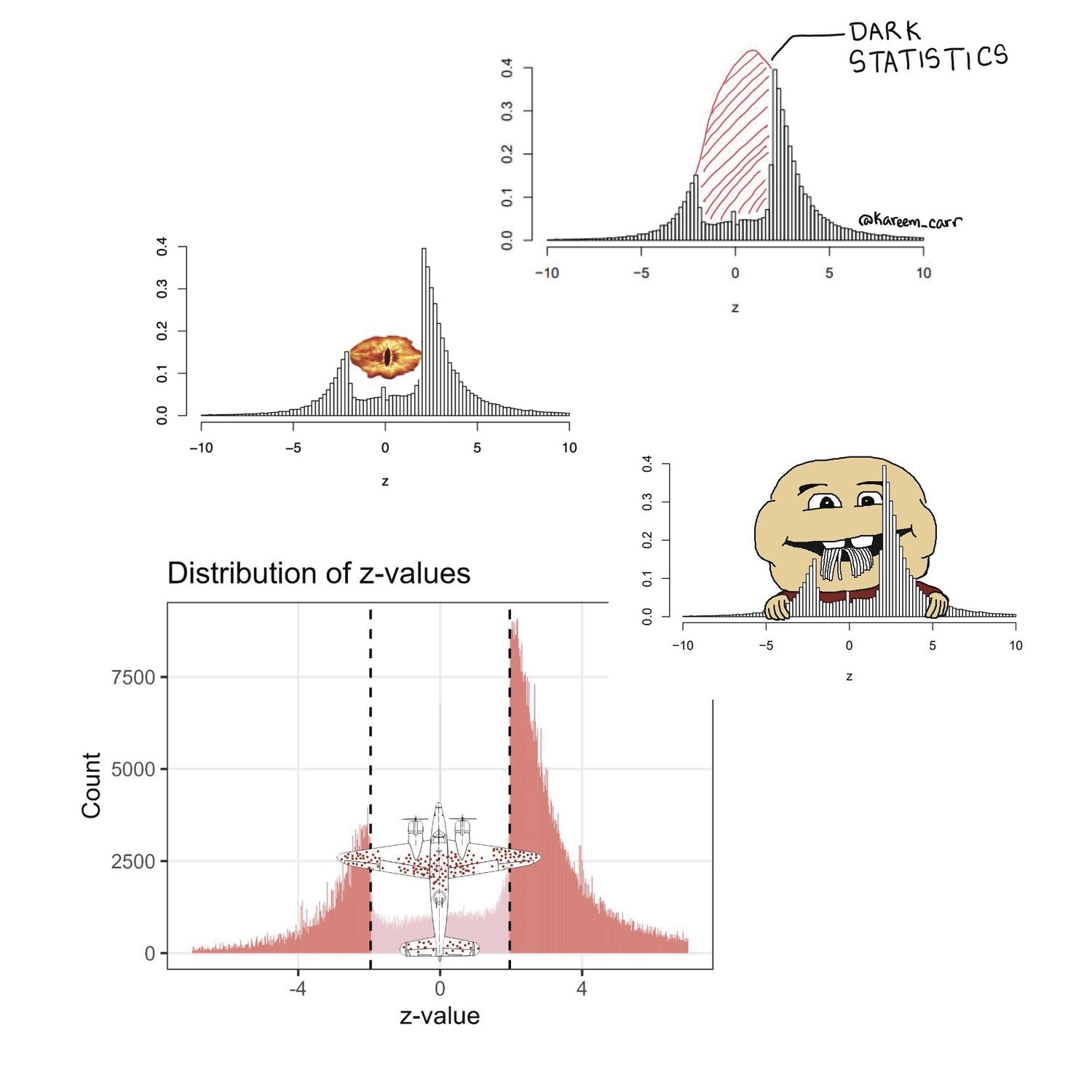
This is Erik. Five years ago, I wrote a short paper about The significance filter, the winner’s curse and the need to shrink (with Eric Cator). The main purpose was to publish some mathematical results for later reference. To make the paper a little more interesting, we wanted to add a motivating example. I came across a paper by Barnett and Wren (2019) who scraped more than a million confidence intervals of ratio estimates from PubMed and made them publicly available. I converted the confidence intervals to z-statistics, made a histogram, and was struck by the lack of z-statistics between -2 and 2 (i.e. non-significant results).

load(url("https://github.com/agbarnett/intervals/raw/master/data/Georgescu.Wren.RData"))
d=complete[complete$mistake==0,]
L=log(d$lower)  # take the log because these are ratio estimates
U=log(d$upper)
estimate=(L+U)/2
stderror=(U-L)/(2*1.96)
z=estimate/stderror
hist(z[abs(z)<10],100)

Richard McElreath noticed the figure, snipped it from our paper and posted it on Twitter. Next, it was picked up by several (relatively) large accounts; Harlan Krumholz, Inquisitive Bird, Kareem Carr, John Holbein, Cremieux and  Nicolas Fabiano. Just 2 weeks ago John Holbein re-upped his earlier post and got another few thousand likes. The histogram is also quite popular with bloggers, see here, here, here, here, here, here, here, here, here, here, here and here. Adrian Barnett and David Borg wrote a blog post with their own version of the histogram. Several memes were also created.

For the fifth anniversary of the histogram, I wanted to react to a few typical comments. For example, Adriano Aguzzi commented:

Let’s not hyperventilate about this. It’s in the nature of things that negative results are rarely informative and therefore rarely published. And that is perfectly legitimate.

It is disappointing – to say the least – that many people still fail to see the problem of distorting the scientific record by selectively reporting and publishing results that meet p<0.05.

Another typical comment (Simo110901):

I don’t think this is inherently bad, a part of this bias certainly comes from publishing bias, but a significant part (hopefully the majority) could be that researchers are often really good at formulating educated guesses and therefore able to reject null results in most cases.

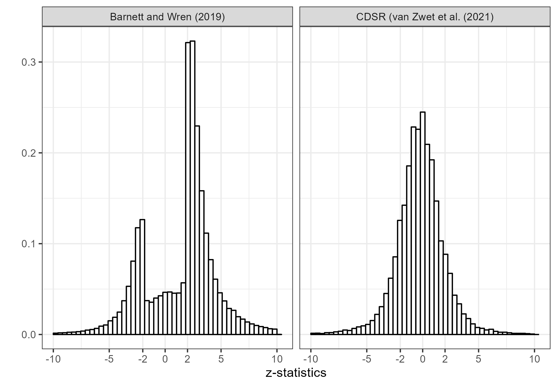
Many other commenters also believe that the lack of non-significant results is due to researchers’ ability to size their studies exactly right to obtain statistical significance with minimal undershoot. This is very unlikely. In the figure below, I compare the z-statistics from Barnett and Wren (2019) to a set of more than 20,000 z-statistics of the primary efficacy endpoints of clinical trials from the Cochrane Database of Systematic Reviews (CDSR).

d=read.csv("https://osf.io/xq4b2/?action=download")
d=d %>% filter(RCT=="yes",outcome.group=="efficacy", outcome.nr==1, abs(z)<20 ) 
d=group_by(d,study.id.sha1) %>% sample_n(size=1)        # one outcome per study 
hist(d$z[abs(d$z)<10],50)


The histogram from the CDSR (right) shows no appreciable gap. I can’t know for sure why that is, but would guess it’s due to the fact that clinical trials are serious research. They are usually pre-registered in the sense that they have a protocol which was approved by some Institutional Review Board. They are expensive and time-consuming, so even if they are not significant it would be a shame not to get a publication out of them. Finally, it would be unethical to the participants not to publish.

Another typical comment (Daniel Lakens):

This is not an accurate picture of how biased the literature is. The authors only analyze p-values in abstracts.

Barnett and Wren (2019) collected z-statistics from both abstracts and full text sources. The full text data are available for papers that are on PubMed Central. There are 961,862 abstracts and  348,809 full-text sources. Below, I show the z-statistics separately. The distributions are remarkably similar, although there is a slightly higher proportion non-significant results from the full texts

Any automated scraping algorithm is bound to miss some things. It’s quite possible that non-significant results that are not in the abstract or main text are still reported in separate tables, appendices and supplements. However, it doubt that that’s the reason for the huge gap. I’m quite convinced that the z-statistics from PubMed really do provide strong evidence of publication bias against non-significant results in the medical literature. However, it should be noted that the underrepresentation of z-statistics between -2 and 2 is probably not only due to publication bias, but also due to authors not reporting confidence intervals for non-significant results. Of course, that is still not a good thing.