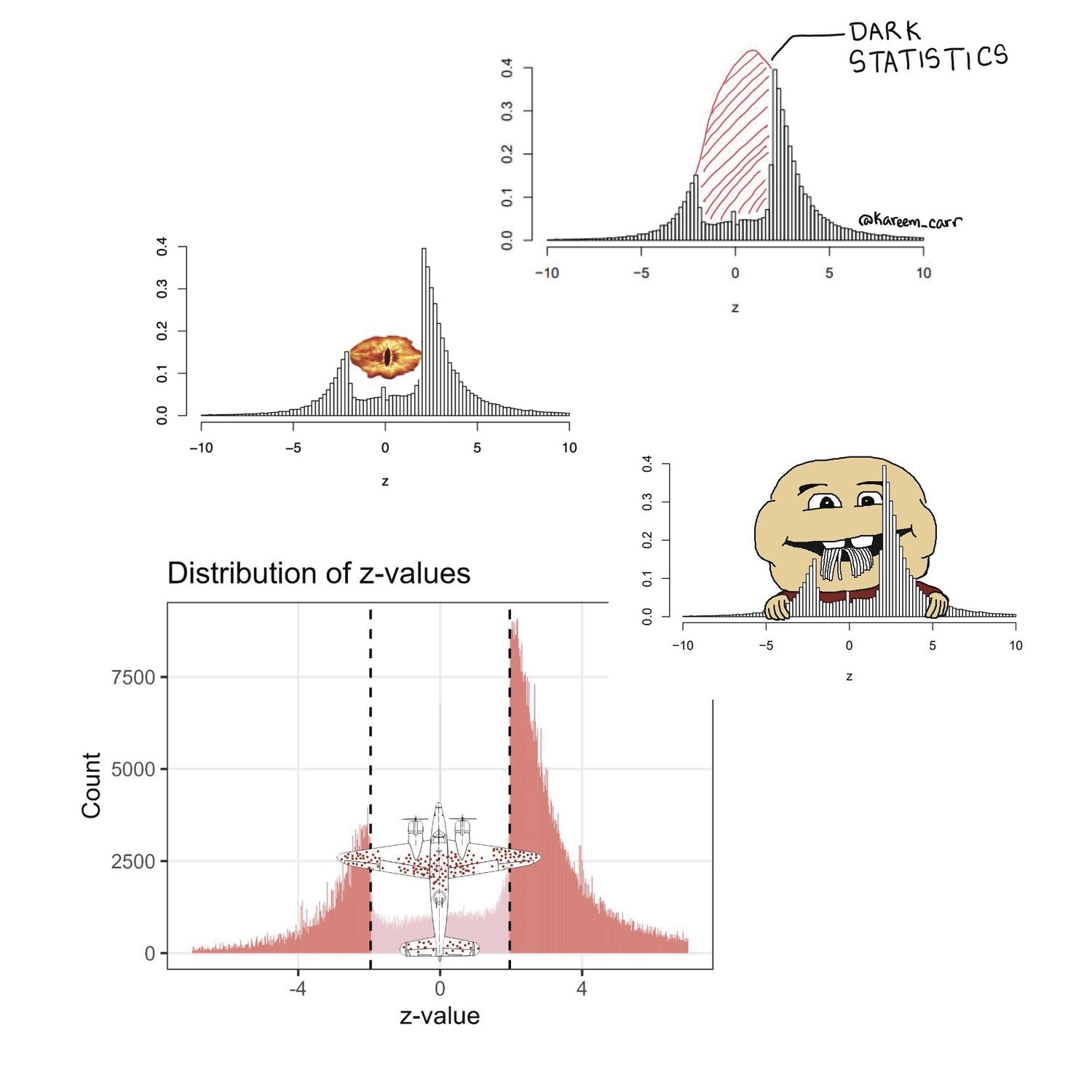
This is Erik. Five years ago, I wrote a short paper about The significance filter, the winner’s curse and the need to shrink (with Eric Cator). The main purpose was to publish some mathematical results for later reference. To make the paper a little more interesting, we wanted to add a motivating example. I came across a paper by Barnett and Wren (2019) who scraped more than a million confidence intervals of ratio estimates from PubMed and made them publicly available. I converted the confidence intervals to z-statistics, made a histogram, and was struck by the lack of z-statistics between -2 and 2 (i.e. non-significant results).
load(url("https://github.com/agbarnett/intervals/raw/master/data/Georgescu.Wren.RData"))
d=complete[complete$mistake==0,]
L=log(d$lower)  # take the log because these are ratio estimates
U=log(d$upper)
estimate=(L+U)/2
stderror=(U-L)/(2*1.96)
z=estimate/stderror
hist(z[abs(z)<10],100)

Richard McElreath noticed the figure, snipped it from our paper and posted it on Twitter. Next, it was picked up by several (relatively) large accounts; Harlan Krumholz, Inquisitive Bird, Kareem Carr, John Holbein, Cremieux and Nicolas Fabiano. Just 2 weeks ago John Holbein re-upped his earlier post and got another few thousand likes. The histogram is also quite popular with bloggers, see here, here, here, here, here, here, here, here, here, here, here and here. Adrian Barnett and David Borg wrote a blog post with their own version of the histogram. Several memes were also created.
For the fifth anniversary of the histogram, I wanted to react to a few typical comments. For example, Adriano Aguzzi commented:
Let’s not hyperventilate about this. It’s in the nature of things that negative results are rarely informative and therefore rarely published. And that is perfectly legitimate.
It is disappointing – to say the least – that many people still fail to see the problem of distorting the scientific record by selectively reporting and publishing results that meet p<0.05.
Another typical comment (Simo110901):
I don’t think this is inherently bad, a part of this bias certainly comes from publishing bias, but a significant part (hopefully the majority) could be that researchers are often really good at formulating educated guesses and therefore able to reject null results in most cases.
Many other commenters also believe that the lack of non-significant results is due to researchers’ ability to size their studies exactly right to obtain statistical significance with minimal undershoot. This is very unlikely. In the figure below, I compare the z-statistics from Barnett and Wren (2019) to a set of more than 20,000 z-statistics of the primary efficacy endpoints of clinical trials from the Cochrane Database of Systematic Reviews (CDSR).
d=read.csv("https://osf.io/xq4b2/?action=download")
d=d %>% filter(RCT=="yes",outcome.group=="efficacy", outcome.nr==1, abs(z)<20 )
d=group_by(d,study.id.sha1) %>% sample_n(size=1)        # one outcome per study
hist(d$z[abs(d$z)<10],50)
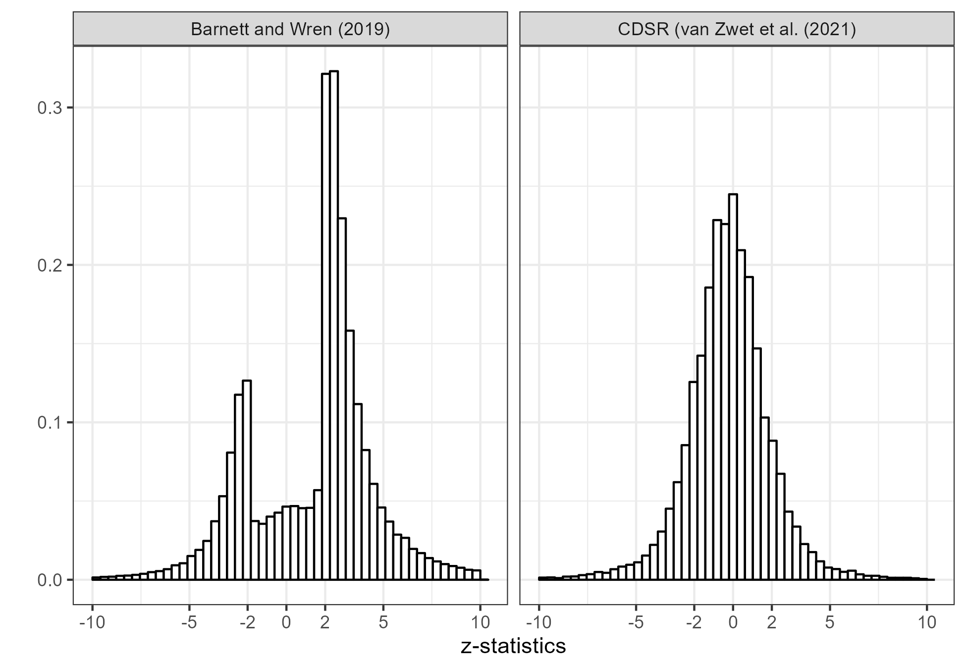
The histogram from the CDSR (right) shows no appreciable gap. I can’t know for sure why that is, but would guess it’s due to the fact that clinical trials are serious research. They are usually pre-registered in the sense that they have a protocol which was approved by some Institutional Review Board. They are expensive and time-consuming, so even if they are not significant it would be a shame not to get a publication out of them. Finally, it would be unethical to the participants not to publish.
Another typical comment (Daniel Lakens):
This is not an accurate picture of how biased the literature is. The authors only analyze p-values in abstracts.
Barnett and Wren (2019) collected z-statistics from both abstracts and full text sources. The full text data are available for papers that are on PubMed Central. There are 961,862 abstracts and 348,809 full-text sources. Below, I show the z-statistics separately. The distributions are remarkably similar, although there is a slightly higher proportion non-significant results from the full texts

Any automated scraping algorithm is bound to miss some things. It’s quite possible that non-significant results that are not in the abstract or main text are still reported in separate tables, appendices and supplements. However, it doubt that that’s the reason for the huge gap. I’m quite convinced that the z-statistics from PubMed really do provide strong evidence of publication bias against non-significant results in the medical literature. However, it should be noted that the underrepresentation of z-statistics between -2 and 2 is probably not only due to publication bias, but also due to authors not reporting confidence intervals for non-significant results. Of course, that is still not a good thing.
Personally, the actual statistics of a clinical trial has always seemed dreadfully boring (for good reasons). The CDSR histogram is such a nice control.
Nice post! As you know, in recent years I’ve used that figure in many talks.
I notice some of the posts you linked described the graph as if it were a “bell curve” or normal (Gaussian); but it isn’t: It’s not only centered above zero, but the upper tail is longer and heavier than a fitted Gaussian. I suspect that the skewing was dampened a bit by inconsistent coding of the direction of the contextual alternative.
Also, some write as if the central drop offs are razor sharp, but there appears to be small pile ups just inside the central interval boundaries (where p is just above 0.05). I attribute that to a phenomenon I’ve observed often enough, where authors appear to have been trying for nonsignificance (“upward P-hacking”) because that’s what they want to report. In contrast to trying for significance (“downward P-hacking”), trying for nonsignificance is rarely discussed; but it’s not that uncommon in certain topics where there are high stakes on what is reported, as when the alternative supports liability claims. An example is explored in detail in Rafi & Greenland (‘Semantic and cognitive tools to aid statistical science: replace confidence and significance by compatibility and surprise’. BMC Med Res Methodol 2020;20:244).
There may also be a bias in selecting an effect size? Suppose some effect can theoretically be between 0 and 1 but that the substantively significant effect sizes are above 0.5. Then, the concerned scientists would experiment only for those large effects with sample sizes with the corresponding powers. Even if all those scientists publish their results, i.e., without publication bias, the published results would have disproportionally more statistically significant results?
This is common in clinical trials when authors believe that a non-signifcant contrast in confounding effects between treatment arms is evidence of equivalence, really absence of bias, between treatment arms.
In reply to Greenland’s comment
Re: “It is disappointing – to say the least – that many people still fail to see the problem of distorting the scientific record by selectively reporting and publishing results that meet p<0.05." Earlier this year, the American Astronomical Society's blog-like *NOVA* research highlights website posted an article marking the 2000th article published in the society's most recently established (micro)journal, *Research Notes of the AAS*. The post is by RNAAS editor/moderator Chris Lintott. RNAAS is a unique publication; it posts only short articles, with at most one figure, and they are moderated by AAS editors rather than peer reviewed. In Lintott's words:
"RNAAS‘s purpose is to get information of interest into the formal record quickly, without paying attention to notability. With a few exceptions (mostly for novel theory, which really does need peer review), if you have an astronomical result (even, perhaps especially, a null result), observation, or fact to write down, RNAAS will take it."
Note in particular the mention, "especially," of null results. I wonder how many other disciplines have a journal that specifically welcomes null results. I don't know how successful RNAAS has been as a home for null results; the papers I've read there have mostly been on useful bits of methodology or simple algorithms. My lone RNAAS paper is a description of a new (I think!) distribution useful in astronomy (the "break-by-one gamma distribution"). I'm glad AAS has RNAAS.
A quick AI search yielded some journals that encourage “null results”, for example the Journal of Articles in Support of the Null Hypothesis, Journal of Negative Results – Ecology and Evolutionary Biology, and Journal of Pharmaceutical Negative Results. I have no experience with these journals though. Apparently Discover Journals (Springer Nature) and APA Journals also welcome null results but, again, I don’t know how that works out in practice.
Erik:
The journals Psychological Science and PNAS have traditionally prioritized null results. They just have the convention that their null results are reported as “statistically significant,” that’s all.
One thing I always wondered about this plot: Wouldn’t we expect the distribution of p values to be centered around 0 iff the average effect size is exactly 0? I understand that the CDSR database seems to be nicely centered around 0, but clinical trials are quite a few steps of generalization away from the research they are based on. Most of the research that I am familiar with, we have (more-or-less established) theories that make predictions, often paired with some form of extension, so that there is prior evidence that the (true) effect size is not 0. If that is the case, then the way I understand it, the distribution should not be centered around 0. Someone please enlighten me if my intuition is wrong.
To my eye the z-stats look like they are centred slightly to the right of zero.
The Pubmed z-stats are a little off to the right, and the CDSR z-stats to the left. In the case of the CDSR, I know that we’re always comparing treated to control. However, it’s not clear if a numerically positive or negative effect of the treatment is beneficial for the patients. For example, a numerically positive effect could mean more deaths or more cures for the treated.
I agree. People aren’t going to waste time on treatments that they don’t think will work. You’d also expect them to size a trial for the treatment effect they expect to get. So, the z’s are going to be expected to be outside pm 2 by design. It would be interesting to see a histogram of z’s over time because you’d expect the low hanging fruit to be tried first i.e. the spread of the z’s will get narrower over time.
Clinical trials are different because you just don’t want to show the new treatment works but you also want to show that 1) any side effects don’t crop up more in the new treatment group and that 2) the new treatment group doesn’t differ on any demographic variables compared to the control/old treatment group i.e. no obvious lurking variables. You’d hope to get more non-significant results than significant results i.e. randomisation worked (ns), the treatment worked (s) and the new treatment doesn’t do more harm (ns).
Anon:
You write, “the z’s are going to be expected to be outside pm 2 by design.” But, in a study without selection, the design doesn’t determine z. The observed z is a convolution of the distribution of the true signal-to-noise ratios and a unit normal distribution. Aim for z=2 and, even if your guessed treatment effect is correct–and it won’t be–your z’s could easily be anywhere from 0 to 4. Then consider that your guessed effect size is just a guess, and it blurs the distribution even more.
It’s not clear whether the CDSR z-values you plotted are from individual trials within the SRs, or from meta-analysis of the primary endpoint in the SRs.
Either way, you’d expect the much more plausible distribution of z-values because systematic reviews of a randomisable question attempt to find all the RCT evidence. Clinical trials are not one-and-done, the regulatory agencies (or guideline writers for non-drug interventions) require confirmation before licensing (or recommending) a new intervention, and both Pharma and the public/charity sectors do “post-marketing” trials because regulatory trials rarely answer the questions clinicians need answering before they change practice.
So, we will usually have several trials, done by several different organisations. SRs define their own primary and secondary outcomes, based on importance to clinical practice, so they will find anything buried in supplementary materials and may ask authors to supply unpublished results.
I don’t know the full history of the gap-tooth plot. If it is based on p-values from RCTs in PubMed, the source material is similar to that of the CDSR. As far as I can tell, without digging deeper than I have time for right now, the difference is in the method, not the raw materials.
The CDSR z-statistics are from individual trials within the systematic reviews (SRs). The z-statistics from Barnett and Wren are an automated scrape of the confidence intervals ofratio estimates within the PubMed database. That is quite different!
If we wanted to model the process that generated the intervals, it should also account for the sample size choice. People choose sample sizes they anticipate will yield “significance”, balanced against the cost of collecting data. Ie, the “optimal” result for publication purposes is to spend just enough to get barely significant results.
Since the null hypothesis was essentially always false in these studies, I would expect perfect researchers (doing perfect preliminary power analyses) to never do a study that resulted in non-significant results. Ie, theoretically the ideal histogram would be bimodal with peaks at exactly -1.96 and 1.96. Then starting from that we would need to add some padding, dispersion, etc to account for rounding and imperfect researchers. Likely other cutoffs (p < 0.01) need to be modeled as well.
I made a histogram that roughly shows what I mean. By mirroring across 2 and -2, we can see the apparent publication bias effect is somewhat less when the “bimodal theory” is used rather than assuming a roughly normal distribution should be expected:
https://image2url.com/images/1763238102927-4190a8b1-7007-433f-90fa-dfc572723506.png
R code (run after Andrew’s in the OP to get the original z vector):
# Mirror across significance threshold
z2 = c(z, -4 – (z[z 2]))
# Plot
par(mfrow = c(1, 1))
hist(z[abs(z)<10], 100,
main = "",
xlab = "z-statistic",
freq = F,
col = rgb(1, 0, 0, .5))
hist(z2[abs(z2)<10], 100,
xlab = "z-statistic",
freq = F,
col = rgb(0, 0, 1, 0.3),
add = T)
legend("topleft",
legend = c("Original", "Bimodal Theory w/o Publication Bias"),
bty = "n",
lwd = 6,
col = c("Red", "Blue"))
Looks like it tried to parse it as html. Last try for the important part:
# Mirror across significance threshold
z2 = c(z, -4 – (z[z < -2]), 4 – (z[z > 2]))
z-statistics have a standard normal noise component, so their distribution cannot have the sharp drop-offs we see in the PubMed data (without selection).
Suppose the (unknown) true effect of some treatment is mu and we have a normally distributed, unbiased estimate y with standard error s. In other words, y has the normal distribution with mean mu and standard deviation s. The z-statistic is z=y/s and the signal-to-noise ratio is SNR=mu/s. It follows that z has the normal distribution with mean SNR and standard deviation 1.
Now suppose your perfect researcher does know mu, and decides he/she wants 80% probability of a significant result (or 90% or 99% or whatever). Then he should choose the sample size such that the SNR is 2.8 (or -2.8) because
pnorm(-1.96,2.8,1) + 1 – pnorm(1.96,2.8,1)
is 0.8.
Now suppose all the researchers in some field do the same; they all arrange their experiments to have SNR=2.8 or -2.8. Then the distribution of their z-statistics would be some mixture of two normal distributions; one with mean -2.8 and standard deviation 1 and one with mean 2.8 and standard deviation 1. That is indeed a bimodal dsitribution.
z=c(rnorm(10000,-2.8,1), rnorm(10000,2.8,1))
hist(z,50)
In reality, however, researchers don’t know the true effect. And even if they did, they would not be able to get the power (SNR) they want because of practical limitations (time, money and the availability of participants). As a result, the distribution of the z-statistics across some field of research is the convolution (sum) of some distribution of SNRs and the standard normal. And that’s what we see in the Cochrane data.
It threw me off at first, but check how Andrew calculated it in the OP. These “z-statistics” are calculated from confidence intervals published in papers, which depend on sample size. This can have any distribution. There is nothing forcing any normal distribution.
Starting from the premise that the null hypothesis being tested is always false, every result between [-2, 2] in these charts represents a failed power analysis. Ie, its certainly possible to generate something like the Cochrane distribution from the “bimodal theory”. It just means people are very inefficient when designing studies, or are trying *not* to get significance (because it was about vitamins or whatever).
I’m actually the OP, not Andrew.
z-statistics always depend on the sample size, whether they are calculated directly from the effect estimate and its standard error, or from confidence intervals.
You’re right that there’s no reason why z-statistics should have a normal distribution across a field of research. For example, the distribution of z-statistics across the CDSR has bigger tails than normal. However, it’s not true that z-statistics can have any distribution; it must be the convolution of some distribution of SNRs and the standard normal. Therefore, it must have a certain smoothness.
In the CDSR, we find that smaller z-stats are more common than larger ones. In other words, the distribution of the absolute value of the z-stats is decreasing. This implies that the distribution of the absolute SNRs is also decreasing. We ascribe that to some anthropic principle, i.e. some interplay between optimism and limitations of time, money and participants. You know how it goes: the statistician calculates n=200 for 80% power, and the researcher says they can only manage n=100.
There are many other fields of research where we find a similar decreasing distribution of the absolute z-stats. We’ll publish about that soon!
Anon:
What Erik said. There is no way that an underlying bimodal distribution of effect sizes would give a distribution of z-statistics such as displayed in that graph. It’s true that the convolution isn’t exactly with a standard normal, but it’s close enough that this noise convolution would smooth out the histogram. Absent selection, you would not see a sharp boundary at z=2.
As Erik wrote in his post, you’ll sometimes see the counter-argument that this selection on statistical significance is ok, after all everybody knows that this is done, and it’s only the statistically significant results that should be reported. The trouble is that (a) selective reporting throws away information, to the extent that later researchers and decision makers are relying on what is published, not going back to the raw data; (b) in real life, people use published values as estimates of effect sizes and they use published confidence intervals as summaries of inferential uncertainty, without even trying to correct for the selection bias. As a result, extreme overestimates proliferate on their own and get piped into meta-analyses. We’ve discussed many many examples over the years in this space.
Sorry Eric, I didn’t see it was your post. To address both of your points:
There is selection in this “bimodal theory”. The researchers can select which study to perform to begin with, in particular the sample size which controls the confidence interval. Perfect researchers spending exactly as much as needed on sample size could indeed result in that graph.
Of course, I don’t claim there are perfect researchers or that publication bias isn’t rampant. Just that people definitely do try to choose their sample size to get significance and this should affect what we expect this distribution to look like in the absence of publication bias.
It also changes the interpretation of what a “good” distribution would be. The Cochrane one doesn’t look good to me. That is how lots of inconclusive under-powered studies would appear.
No, without section *on z-statistics* you cannot get that sharp drop-off. Without selection, the distribution of z-statistics must be at least as smooth as the standard normal no matter how clever the researchers choose their sample sizes.
So when I did preclinical research we add sample size in batches of e.g., 10, then would continue until either running out of money (somewhat dependent on the trend) or getting significance. Taken to the extreme someone could add one new datapoint at a time until either threshold is hit. And there was always going to be some difference.
Do your assumptions/calculations address this case? I think your theory here deserves its own post on the blog btw. Obviously it is counterintuitive to multiple commenters here.
Anon:
That’s an interesting example. I think Erik would characterize it as “selection,” but I agree that it’s different than the usual pattern of selection, which is to run the experiment, get lots of data, and fish out the statistically significant results.
In your example, I’d say it’s selection on a sequence of z-statistics.
It’s a good idea to write a separate post about this. I’ll give it a try!
Thanks. However, I’m not so concerned about the term “selection”, rather that we model the actual process that generates the data in those charts.
Afaict, the general consensus is that it “should” look something like a normal distribution. This seems like saying the literature *should* (in a prescriptive sense) be dominated by inconclusive underpowered results. No one would notice this chart in that case.
I’m not saying it should look like a normal distribution. The z-stats from the CDSR also don’t follow a normal distribution; their distribution has much heavier tails than normal.
I am saying the distribution of z-stats should be at least as smooth as the standard normal distribution. Therefore, that sharp drop-off between -2 and 2 must be due to selection on statistical significance. This selection can happen in many different ways, including your example of increasing the sample size until significance.
I’m also providing “circumstantial evidence” by comparing the z-stats from PubMed to those from the CDSR. Researchers who run clinical trials would love to get statistical significance with minimal time, money and participants. And yet they are not able to avoid z-stats between -2 and 2 like we see in the PubMed data.
If you condition publication on a feature of the data, then finding that feature in a publication has no signal value.