Over the next posts, let’s dig into Michael Bailey‘s A New Paradigm for Polling and the commentary it got from other wonderful survey statisticians. In this post, let’s get introduced to the response instrument, and see what these folks have to say about it.

Bailey begins:
the polling field needs to move to a more general paradigm built around the Meng (2018) equation that characterizes survey error for any sampling approach, including nonrandom samples.
We discussed Meng 2018 “Statistical Paradises and Paradoxes” in this blog series here.
Most of what we’ve discussed so far (e.g. poststratification, weighting) assumes that within groups based on covariates X, response R is independent of outcome Y. Random sampling (within X) achieves this.
In Section 4, Bailey looks at some methods for when R might depend on Y (within X), a “nonrandom” paradigm. These methods rely on a response instrument Z: a variable that affects the probability of response R but does not directly affect the outcome of interest Y.
For example, let Z = 0 if someone is forced to discuss politics (“high response protocol”), and Z = 1 if they are given the choice to discuss politics or opt out and discuss sports (“low response protocol”). From Bailey 2025 (with my additions in green):

Intuitively, the response instrument helps because we can compare observed Y between low versus high response protocols, which gives information about the dependence between Y and R. How this translates to an estimate of population Y depends on methods and assumptions Bailey doesn’t fully dive into here.
Sharon Lohr’s comments describe a sufficient assumption: no interaction between outcome Y and instrument Z in the model for response R. Confusingly, she uses “X” instead of “Z” for the instrument, so I’ve edited below:
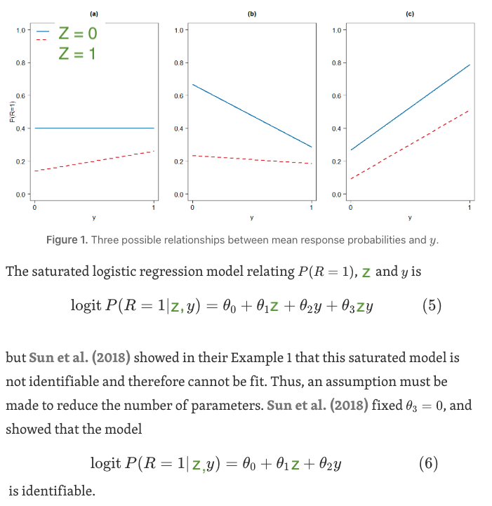
All three models in Figure 1 perfectly fit the data. In Figure 1(a), the high response protocol (Z = 0) is “random” (R does not depend on Y), so our usual methods work. In Figure 1(c), there is no Z*Y interaction in the response model, so the response instrument methods work. In Figure 1(b), it isn’t clear what to do.
Perhaps we should propagate uncertainty about these assumptions to our final results. Rod Little’s comments include a suggestion to “use Bayesian modeling, including a prior distribution for unidentified parameters.” Has anyone seen a good example of Bayesian modeling using response instruments ?
In his comments, Shiro Kuriwaki says that randomized instruments “give us leverage in the face of unobservable confounders, but no leverage comes for free.” He advocates more research into these methods. Agreed !
We’ve been focused on the randomization instrument Z. But we can’t forget about the response R and how its dependence on Y differs with different survey recruitment protocols (e.g. web versus text), see Sharon Lohr’s comments. And conditioning on more covariates X increases the plausibility that Y and R are independent. So instead of pursuing a randomization instrument, we could focus on improved recruitment protocols and enlarging our set of covariates X. Thoughts ?
p.s. Bailey’s post also clarifies why Raphael Nishimura doesn’t like the term “representativeness”, see this blog comment: it’s too vague, and can be used to mean “matches some population demographics”, which may not guarantee much about the outcomes of interest Y.
Gustavo and I wrote a short discussion of the Bailey paper that was published in same issue of that journal. We wrote:
Our paper has some pretty graphs, too. Maybe I’ll post something on it directly!
Thanks, Andrew ! I’d like to write the next posts covering the other discussions of Bailey’s post, including yours of course. In this one I focused on the response instrument, which I think isn’t directly covered your paper ?
Do you think this is true also of polls that recruit in other ways, e.g. online platforms that pay people to take surveys on all topics, and politics is just in that mix ?
Shira:
I can’t be sure, but, yes, I would guess that polls in general, including those from online panels, oversample people who are interested in politics.
In equation 6, why is there no comma between z and y and instead, there is a blank space? Is this some sort of convention to indicate that the product term, zy, is not allowed in the model.
Ah good catch, paul ! No, this is because I was editing a screenshot from Sharon Lohr’s comments very sloppily. Let me fix that :)
Thanks Shira for digging into this.
My big picture take is that our models should reflect the nature of the problem. Every single pollster recognizes that R may depend on Y — and that this is likely a cause of “misses” regarding Trump over the last decade (and chronic problems in estimating turnout from polls etc). So why should be be content with models that assume that away?
You’ve provided a nice introduction to randomized response instruments. For folks new to the concept, I like to start with the “tilted fish” (see https://hdsr.mitpress.mit.edu/pub/ejk5yhgv/release/4). With ignorable nonresponse (MAR) the average of Y is the same for all levels of response interest. (Each dot is a person; dots on the right really love to respond.)
With non-ignorable nonresponse (MNAR) the average of Y differs by level of response interest. A randomized response instrument varies the (effective) response instrument. Seeing the values of Y differ across treatment groups would be consistent with non-ignorable nonresponse. Seeing no difference would be consistent with ignorable nonresponse.
As Kuriwaki, Lohr and other point out, randomized response instruments require assumptions (I go into more detail in the 2025 paper that you linked to). But let’s not forget that conventional MAR based models assume that R is independent of Y — a potentially strong assumption. Randomized response instruments can allow the effect of a response instrument to vary by X, but not Y.
I don’t think randomized response instruments are a magic bullet or final word, but they do allow us to stop assuming MAR and they always (afaik) help reduce bias in polling based estimates of turnout and often suggest that Trump numbers are too weak due to non-ignorable nonresponse.
I hope there’s a lot more research on the topic — and more broadly, that we move beyond MAR limits. I’ve got a paper using panel data — we can literally observe differences in response interest by individual and we definitely see differences in Y (e.g., turnout or Trump vote) associated with these differences, even when controlling for X.
Thank you, Michael !
I do feel that the MAR assumption can be made more plausible if we work on improved recruitment protocols and enlarging the set of covariates X that we adjust for (Andrew and Gustavo’s comments relate to this). I’m not sure how to think about pursuing those lines of research versus pushing beyond-MAR. Both seem important !
Regarding specific models for differential nonresponse, I recommend The mythical swing voter from 2016 and Modeling differential nonresponse in sample surveys from 1998.
Thanks, Andrew !
Indeed, enlarging the set of covariates X can make a big difference, as you point out in The mythical swing voter: