The other day we discussed my struggles fitting models to the golf putting data.

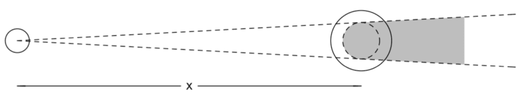
My earlier modeling was mostly a success—it’s a popular example, it’s a Stan case study, and it’s in our workflow article. We had an initial dataset that we can fit with a simple one-parameter geometry-based model:

Then we got new data where the first model doesn’t fit but we can fix by following Mark Broadie’s suggestion and adding just one more parameter to capture a little bit more of the geometry of the problem:

That was all good but we had convergence problems fitting this model in Stan, and the only way I could get it to fit smoothly was to add a fudge factor, an independent error term at each distance. Including this extra error did not bother me—after all, we would not expect an simple model to fit real data perfectly—but I was annoyed that, to add this error term, I needed to approximate the binomial likelihood with a normal distribution. Such an approximation would give problems going forward if we wanted to model the probability of success given players, golf courses, and weather conditions, in which case we’d have lots of cells with just 1 or 2 observations so the normal approximation wouldn’t work.

So I tried a direct approach, adding an error term to the modeled probability of success—but that couldn’t be done on the probability scale because then the probability could go below 0 or above 1, so I tried an additive error on the logistic scale; in Stan:

p = inv_logit(logit(p_angle .* p_distance) + sigma_eta*eta);

Here, p_angle .* p_distance is the predicted probability of success (the probability of getting both the shot angle and the shot distance within tolerance), and sigma_eta*eta is the vector of errors (with eta given a normal(0,1) prior and sigma_eta representing the scale of the errors). The logistic and inverse logistic transformations keep the probabilities bounded between 0 and 1.

But it didn’t work! Convergence problems again.

And that’s where we were a few days ago. Stuck! Stuck stuck stuck.

There were various suggestions in comments, but none were directly helpful, until this came from Kj:

The problem seems rooted in the model needing the shortest putts probability to be very close to 1 in order to fit the rest of the data. Before the normal hack, the (poorly sampled) model estimates the probability of the shortest putts to be 10^9 in logit space.

The normal hack applies to probability space, and there the error is tiny, so it works fine. But if you look at the error in logit space, the fit remains really bad.

And I was like, Aha! Here’s a solution: a three-parameter model that scales all the probabilities down from 1:

data {
  int J;
  array[J] int n;
  vector[J] x;
  array[J] int y;
  real r;
  real R;
  real overshot;
  real distance_tolerance;
}
transformed data {
  vector[J] threshold_angle = asin((R-r) ./ x);
}
parameters {
  real<lower=0> sigma_angle;
  real<lower=0> sigma_distance;
  real<lower=0, upper=1> epsilon;
}
model {
  vector[J] p_angle = 2*Phi(threshold_angle / sigma_angle) - 1;
  vector[J] p_distance = Phi((distance_tolerance - overshot) ./ ((x + overshot)*sigma_distance)) -
               Phi((- overshot) ./ ((x + overshot)*sigma_distance));
  vector[J] p = p_angle .* p_distance * (1 - epsilon);
  y ~ binomial(n, p);
  [sigma_angle, sigma_distance] ~ normal(0, 1);
}

The key is to make it a multiplier that has to be less than 1. This eliminates the problem with the boundary and the need for the logit.

Success! I’m so happy. Here’s the fit:

       variable        mean      median    sd   mad          q5         q95  rhat ess_bulk ess_tail
 lp__           -363841.724 -363841.000 1.311 1.483 -363844.000 -363840.000 1.000     1636       NA
 sigma_angle          0.018       0.018 0.000 0.000       0.018       0.018 1.002     1905     2165
 sigma_distance       0.080       0.080 0.001 0.001       0.079       0.081 1.002     1659     1859
 epsilon              0.001       0.001 0.000 0.000       0.001       0.001 1.002     1545     1493

I’m not sure what’s going on with the tail effective sample size; we’ll have to look into this. I suspect it’s caused by some rounding error. Doesn’t really matter, though.

The above model fits the data in the sense of going through the data points, but it’s still just a three-parameter model so to really do things right we might still want to add an error term. We can do this, using the same principle of making the errors multiplicative and constraining them to fall between 0 and 1:

data {
  int J;
  array[J] int n;
  vector[J] x;
  array[J] int y;
  real r;
  real R;
  real overshot;
  real distance_tolerance;
}
transformed data {
  vector[J] threshold_angle = asin((R-r) ./ x);
}
parameters {
  real<lower=0> sigma_angle;
  real<lower=0> sigma_distance;
  real<lower=0> sigma_epsilon;
  vector<lower=0, upper=1>[J] epsilon;
}
model {
  vector[J] p_angle = 2*Phi(threshold_angle / sigma_angle) - 1;
  vector[J] p_distance = Phi((distance_tolerance - overshot) ./ ((x + overshot)*sigma_distance)) -
               Phi((- overshot) ./ ((x + overshot)*sigma_distance));
  vector[J] p = p_angle .* p_distance .* (1 - epsilon);
  epsilon ~ exponential(1/sigma_epsilon);
  y ~ binomial(n, p);
  [sigma_angle, sigma_distance] ~ normal(0, 1);
}

This is a little bit hacky because we’re using the exponential density for the epsilons and then constraining to be no more than 1, but in practice it will be fine. The scale parameter sigma_epsilon keeps the errors under control. (I tried epsilon ~ normal(0, sigma_epsilon); model and it gave essentially the same results.) We can also augment the model so it computes residuals:

data {
  int J;
  array[J] int n;
  vector[J] x;
  array[J] int y;
  real r;
  real R;
  real overshot;
  real distance_tolerance;
}
transformed data {
  vector[J] threshold_angle = asin((R-r) ./ x);
  vector[J] raw_proportion = to_vector(y) ./ to_vector(n);
}
parameters {
  real<lower=0> sigma_angle;
  real<lower=0> sigma_distance;
  real<lower=0> sigma_epsilon;
  vector<lower=0, upper=1>[J] epsilon;
}
transformed parameters {
  vector[J] p_angle = 2*Phi(threshold_angle / sigma_angle) - 1;
  vector[J] p_distance = Phi((distance_tolerance - overshot) ./ ((x + overshot)*sigma_distance)) -
               Phi((- overshot) ./ ((x + overshot)*sigma_distance));
  vector[J] p = p_angle .* p_distance .* (1 - epsilon);
}
model {
  epsilon ~ exponential(1/sigma_epsilon);
  y ~ binomial(n, p);
  [sigma_angle, sigma_distance] ~ normal(0, 1);
}
generated quantities {
  vector[J] residual = raw_proportion - p_angle .* p_distance;
}

We needed to move some things into the transformed parameters block so they’d be accessible in the generated quantities calculation. Also, we compute residual relative to p_angle .* p_distance, not relative to p, because the whole point is to look at the fit of two-parameter model fits. The error term epsilon is not part of the prediction, in this sense, even though it would appear to be so in the usual framework of the Bayesian model, for example when computing elpd etc.

Anyway, here’s a plot of the fitted model and the posterior mean of its residuals:

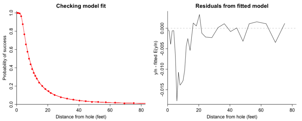
This looks a little bit different from our residual plot before:

Our new plot looks a little bit worse, actually! But I guess it’s a price I’m willing to pay to have a model that is more mathematically coherent.

Hmmm, this gets me wondering . . . What are the residuals from our three-parameter model above, the one where p = p_angle .* p_distance .* (1 – epsilon);, so that there’s a fixed downward multiplier? Let’s take a look:

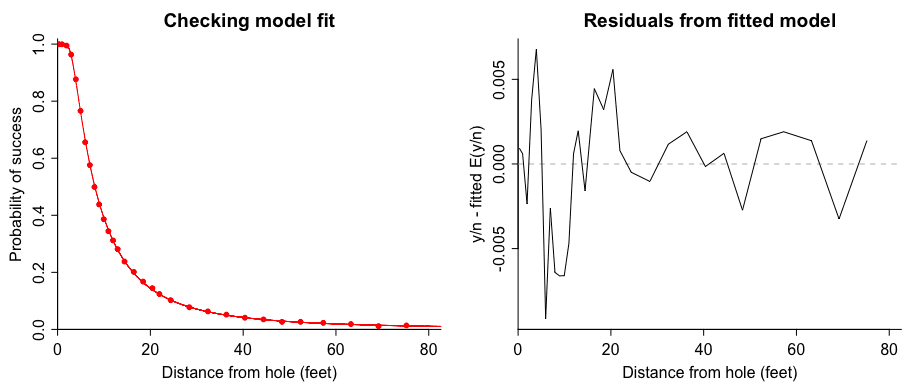
Hey! This looks fine. So I’m inclined to just stop here for now and not bother with that model with the separate epsilon for each distance.

As has been discussed in the comment thread, there are lots of ways this model could be improved, but now we have a simple three-parameter model that fits the data without that normal-approximation hack, so this is what I’d start with going forward, then allowing these parameters to vary by golfer, hole, and weather condition.

And here are the files.