Start by reading the golf case study; it’s also in section 10 of the workflow paper.
The final version of the model has a hack, I went in to try to clean it up, and now I’m having problems fitting what should be the cleaner model.
I’m not sure what’s wrong: it could be a problem with my code, it could be a conceptual problem with my model, or it could be what we call “bad geometry,” leading to computational problem that maybe could be fixed with a reparameterization.
Right now I’m in the middle of things, and I thought I’d share that with you. Usually we present completed projects or vague ideas; this time you’ll get to see what it looks like when were partway through working things out.
What we did before
Here’s the story. We have data on success rates of golf putts as a function of distance from the hole, from a bunch of pro tournaments. There are lots of ways these data could be analyzed: you could estimate the abilities of individual players, improvement over time, the difficulties of different courses, the effects of bad weather, etc. Here we keep it simple: we aggregate all the data together to estimate Pr(success | distance from hole), fitting a two-parameter curve based on a simple mathematical model from Mark Broadie in which the golfer’s challenges are to get the angle and distance correct, and there’s error in both: the two parameters correspond to the standard deviations of the errors in angle and relative distance.
The model fits the data pretty well but not perfectly:

Also, annoyingly, the chains do not mix well when the model is fit in Stan. You don’t really see it in the above graph because the poor convergence is all happening in a close neighborhood of the fitted model. The convergence problem is thus not a major practical concern here, but it’s still annoying and it gives us concerns if we were to apply the model going forward. And it’s just a simple two-parameter model? What’s going wrong?
Here are the data for the first few bins of distance (the data came to us in bins; we don’t have the distance and success for every shot):
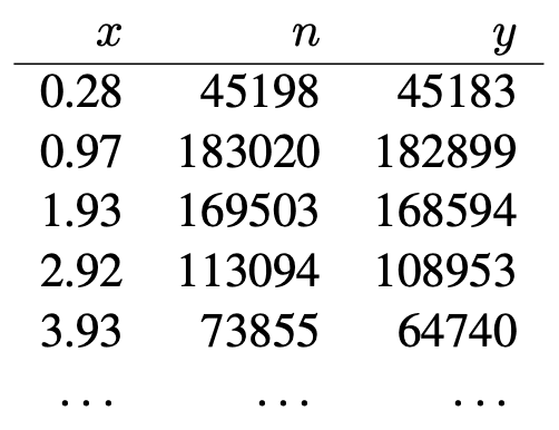
Sample sizes are huge in the initial bins, hence the binomial model tries to fit these points nearly exactly. This in turn makes the model difficult to fit: the constraint for the first few data points essentially ties down the parameters and makes it difficult to effectively more through the posterior distribution.
So I decided I needed to add an error term to grease the wheels of commerce. Here’s what we did:

And the happy result:

Greasing the wheels of commerce—it really worked!
What we’re trying to do
I haven’t yet described where we’re stuck. So far all we did was take a model that wasn’t quite working and add an independent error term to capture modeling error. The independence assumption didn’t quite make sense, but the extra error term did the job in allowing the Hamiltonian Monte Carlo algorithm within Stan to move effectively through the two-dimensional parameter space of interest.
But it was still a hack. What bothered me was the independent error term (although, yes, that could be improved) but, rather, that I needed to resort to the normal approximation. What I really wanted to do was to keep the binomial model and then add the error on the logistic scale or something like that, something to keep the probabilities bounded between 0 and 1. So I put this in the Stan model:
data {
  int J;
  array[J] int n;
  vector[J] x;
  array[J] int y;
  real r;
  real R;
  real overshot;
  real distance_tolerance;
}
transformed data {
  vector[J] threshold_angle = asin((R-r) ./ x);
}
parameters {
  real<lower=0> sigma_angle;
  real<lower=0> sigma_distance;
  real<lower=0> sigma_eta;
  vector[J] eta;
}
model {
  vector[J] p_angle = 2*Phi(threshold_angle / sigma_angle) - 1;
  vector[J] p_distance = Phi((distance_tolerance - overshot) ./
    ((x + overshot)*sigma_distance)) -
    Phi((- overshot) ./ ((x + overshot)*sigma_distance));
  vector[J] p = inv_logit(logit(p_angle .* p_distance) + sigma_eta*eta);
  y ~ binomial(n, p);
  eta ~ normal(0, 1);
  [sigma_angle, sigma_distance, sigma_eta] ~ normal(0, 1);
}
Let me explain. Most of the model is what we had before: it’s a calculation, given the hyperparameters, that your shot’s angular error is small enough and that it’s distance error is small enough that the ball goes in the hole, according to our simple geometric model. We’re assuming the two errors are statistically independent; hence we were using p = p_angle .* pdistance.
In this new version of the model we added the error term, sigma_eta*eta, and to keep everything in the unit interval, we added it to the probability on the logit scale.
The bad news is when fit this new model to our data, it doesn’t work. The console fills up with warnings and the chains don’t mix.
Where we are now
We were able to fit the golf data with a two-parameter model plus an error term, but we needed to use the hack of the normal approximation to the binomial distribution. Sticking the error term on the logistic scale is a hack too, but less of a hack . . . unfortunately it’s giving me computation problems! It could just be something simple that I’m missing in my code, or there could be something deeper going on. I guess the next step in debugging is to see if the model fits ok to data simulated from the model. What to do next depends on what happens with the fake-data check.
Again, the reason for this post is to give a peek behind the curtain and give a sense of what it feels like to be in the middle of things.
If you want to try any of this out, here are the data and code.
P.S. Success! See here.
The model you are using is assuming distances are exact, while there is likely to be measurement error and certainly there is binning. Maybe you should add rounding model for distances? This would mainly have an effect for the very short distances where the probabilities are near 1.
The second thought is that the geometric model fails in very short distances as the motor control for hitting a ball short distance is more difficult and the effect of friction is bigger. Your extra normal term could be explaining these unknown variations.
Aki:
I was assuming that my error model would implicitly pick up all these things, as well as data irregularities not otherwise accounted for. I was ok with this extra error term because our models are always imperfect. It was just annoying that when I tried to put it on the logit scale the computation blew up.
Shouldn’t some (all?) of those sigma parameters be positive constrained? As it is, they just look like normals instead of half normals.
On the original model, shouldn’t distance overshoot tolerance be modeled on the log scale. I haven’t golfed, but judging by my experience with cornhole and carnival games, uncertainty in landing zone seems close to a fixed fraction of distance from target, since it gets harder to control my power the harder I’m throwing.
Somebody:
Yes, they’re all constrained! This is some stupid html bug that eats up the angle brackets, dammit. I went in and fixed this.
Looks like in the downloadable files, the sigma parameters are positive constrained, so it’s not that.
My second thought is maybe you need tighter priors constraining sigma eta parameter to a smaller value. If sigma_eta is around 1, then each eta could be anything and explain any dataset all on its own, and then the high likelihood surface to explore for the two theoretically motivated parameters is massive. This wouldn’t happen in the normal approximation since it’s a single noise parameter.
Somebody:
What you say could be. It’s just funny that I’m having this problem here and I didn’t have the problem when I used the normal distribution hack. I guess the normal distribution ran more easily because the math of the normal allowed us to implicitly integrate out all the error terms.
You obviously don’t believe the assumptions behind the binomial model are correct, so why be so fixated on keeping them?
Instead derive something closer to the reality from scratch. Either way it looks like you will be required to add more parameters, so you may as well do it in a principled way.
Anon:
Sure, there are lots of ways to go. Given that I don’t think the probability is constant within each bin, maybe it would make sense to start by expanding from binomial to beta-binomial (its overdispersed generalization). Even so the model won’t fit perfectly so it could make sense to add some sort of fudge factor. The normal approximation worked so well in part because of the smooth math that allowed us to include this error term without actually adding the errors to parameter space. The point about the logit is that probabilities are constrained to be between 0 and 1. If, for example, we start to do more modeling including variation across golfers and weather conditions, then at some point our data would start becoming sparse, and it would be natural to move to a logit model and I wouldn’t be able to use the normal approximation, so . . . I thought I’d just shift to the logit right now. But it didn’t work, hence my above post. So it’s not that I’m committed to the binomial likelihood; I was just doing what seemed like the logical next step of cleaning the model.
If I understand the model, x is the measured distance to the hole. And it is binned in about 1 ft intervals. So wouldn’t it make sense to add the fudge factor with an error in variables model?
My stan is somewhat rusty but then I believe you would use something like:
vector[J] x2 ~ normal(x, 1);
vector[J] p_distance = Phi((distance_tolerance – overshot) ./
((x2 + overshot)*sigma_distance)) –
Phi((- overshot) ./ ((x2 + overshot)*sigma_distance));
https://en.wikipedia.org/wiki/Errors-in-variables_models
Instead of assuming normal and sd = 1 for the error you could use a uniform distribution or make that another parameter to vary (rather than sigma_eta).
Or how about use the observed n? You can interpolate to get discrete weights. Eg, it looks like putts in the 0.97 ft bin are likely to be skewed higher in the bin.
Use that to generate a set of 0.01 incremented weights +/- 0.5 ft from each bin value then sample from that distribution to get x2.
I think that would be best and could be done with no extra parameters to fit.
Disclaimer: I’m not a statistician, but I’ve done reading on the sports-stats domain for a while.
I would expect there to be a bit of selection bias based on golfer skill — that is to say, the best golfers are more likely to reach the green in better position than worse golfers. This effect is probably swamped at distances quite close to the hole, where you have lots of second putts after near-misses (unless you only look at first putts, I didn’t see that explicitly stated one way or the other).
The other factor that jumps out is that greens aren’t all that large, so the farthest distances you observe can only occur on a subset of greens, which may not be representative in their difficulty.
Stan:
Interesting point. If we break up the data by golfer and golf course, we could see some interesting interactions with distance.
Didn’t mean to submit that yet. I tried running the package, but I can’t manage to get the posteriors package installed. It’s complaining about something called “format_glimpse”
One more edit. That completely bricked my cmdstanr installation because it looks like cmdstanr calls posterior after it calls cmdstan.
P.S. I thought you were going to stop selling my labor through ReCAPTCHA(TM) to pay for spam filtering. I had to click through three of them this time, one reloading in the middle and asking me to do it again. This is getting ridiculous!
P.P.S. Or maybe I should say that I wish I didn’t have to pay for my comments by selling my own labor to ReCAPTCHA.
Bob:
We were told that the captcha thing was necessary or we’d be overwhelmed by spam. I’m not sure how else to do it, but if you have suggestions, please let me know and I can ask our sysadmin.
Rather use hCaptcha, or just put Cloudflare in front of whatever you’re trying to protect (I assume this comment box?) and they’ll do it for you.
Also I think they might even pay you a little for the work your commenters do!
Pre-submit edit: yup just got ReCaptcha’d twice! Actually not sure how Cloudflare would work if you specifically want to protect your “Post Comment” button, but in theory you can set it up so that no bots will even get to see the button.
Pre-submit edit 2: had to do another one after typing the above.
Sort of a vague, meta question: I am a first year PhD student in CS, working on some computational social science problems. What are some references you would recommend for improving the thought process behind model building? I have taken several stats courses, am going through your textbooks on applied regression. But as of now, I would fit it hard to even know where to begin fitting a model like this from scratch!
Jay:
I recommend our Bayesian Workflow article and the Stan case studies.
Try normal_lcdf instead of Phi. There’s some issues see https://github.com/stan-dev/math/issues/2470.
Sean:
Can you try this on my code? I tried it and it didn’t work at all. First I had problems because it seems that normal_cdf and normal_lcdf don’t work with vectors. Then I looped it and it compiled but it just produced a bunch of errors. But maybe I’m just doing something wrong.
It’s not a problem of accuracy but if you want this to work. Add a function and replace `Phi` with `normal_phi`
“`
vector normal_phi (vector x) {
int N = num_elements(x);
vector[N] lp;
for (n in 1:N)
lp[n] = std_normal_lcdf(x[n]|);
return exp(lp);
}
“`
My theory is that the model is not physically sound because the dataset lacks information on the distance the putt (would have) traveled. In principle, the success probability should be the probability of a small angular deviation times the conditional probability that the putt has the “correct” velocity given the angular deviation, whereas `p_distance` in the model is conditional on distance but not angle.
You really need putt-specific information. The correct velocity is asymmetrical in the sense that if the putt is an inch too short, then it is guaranteed to be unsuccessful but if it is a foot or two too long that is fine as long as the putt travels through the center of the hole. However, even the asymmetry is asymmetrical in the sense that if the center of the ball is tangent to the hole, then the putt needs to be almost completely stopped for it to fall in.
My guess is that for short puts it is fairly easy for a golfer to get the velocity correct so that it would go 18 inches past the hole in expectation, with a standard deviation of 8 inches or so. In that case, all of the action is in the angle. But for longer putts, there is more error in the velocity and for very long distances, the golfer may be trying to succeed within two putts.
> the golfer may be trying to succeed within two putts
Oh interesting
Ben:
I agree the model doesn’t have anything on the two-putts thing—I guess that would lower Pr(success) at long distances if the golfer is not even trying to get the ball in in. But the rest of what you’re talking about, regarding the asymmetry and the greater importance of speed when x is higher, that’s implicit in the model as it is.
In any case, this model will always be missing a lot if we’re aggregating golfers, golf courses, and weather conditions. I just remain annoyed that I can fit the data just fine using the normal approximation but it fails when I do what seems to be the natural thing on the logit scale.
I guess I can try the beta-binomial and see what happens, but even that is kind of a hack as it would not work if the data were more granular. I really just want a fudge factor that represents independent modeling errors as a function of distance, and if I can’t use the logit, then how am I supposed to do that using my usual Bayesian toolkit? The weird errors that come when I fit the Stan model makes me think that there’s some sort of weird rounding thing that’s going on and causing the problem, but none of this makes sense to me.
This does seem unfortunate lol. Without the normal approximation there as comparison, I wouldn’t be bothered, but it is there.
I played around with a few things. Didn’t seem to be numerics causing problems.
Because the fudge factor for the normal shows up in the sd, I ended up moving to trying to weight things.
The most successful thing I tried seems to reproduce the same basic fit just without the warnings lol, so maybe that is or isn’t good:
“`
// Compute the log density of each output
vector[J] logp;
for(j in 1:J) {
logp[j] = binomial_lpmf(y[j] | n[j], p[j]);
}
// Weights are:
// -logp (instead of logp) because we want to make sure those low contributors to density to get some extra attention (and high contributors to log density don’t hog all the fun)!
// sigma_eta cause it works (it seems like we can estimate the scale of how much we’re paying attention to different things)
// softmax (instead of inv_logit) because we don’t really have a sense of scales of logps — I guess we could put an intercept
// and do inv_logit? I dunno if it’d work
vector[J] w = softmax(-sigma_eta * logp);
// Add em’ all up!
for(j in 1:J) {
target += w[j] * logp[j];
}
// A prior!
sigma_eta ~ normal(0, 1);
“`
If you plot sigma_eta over warmup it looks like it’s doing some sort of tempering thing (by the time you get to sampling sigma_eta is very small and the weights are even). Of course I could reading diagnostics wrong and this doesn’t actually work. It doesn’t seem to help the prediction really.
I added back in the thing you had here with the logits in the thinking that the better warmup would help the fit work.
And it seemed to! I had some reasonable success with this model:
“`
data {
int J;
array[J] int n;
vector[J] x;
array[J] int y;
real r;
real R;
real overshot;
real distance_tolerance;
}
transformed data {
vector[J] threshold_angle = asin((R-r) ./ x);
}
parameters {
real sigma_angle;
real sigma_distance;
real scale;
real sigma_eta;
vector[J] eta;
}
transformed parameters {
vector[J] p_angle = 2*Phi(threshold_angle / sigma_angle) – 1;
vector[J] p_distance = Phi((distance_tolerance – overshot) ./ ((x + overshot)*sigma_distance)) –
Phi((- overshot) ./ ((x + overshot)*sigma_distance));
vector[J] logit_p = logit(p_angle .* p_distance) + sigma_eta * eta;
vector[J] logp;
for(j in 1:J) {
logp[j] = binomial_logit_lpmf(y[j] | n[j], logit_p[j]);
}
vector[J] w = softmax(-scale * logp);
}
model {
for(j in 1:J) {
target += w[j] * logp[j];
}
eta ~ normal(0.0, 1.0);
sigma_eta ~ normal(0, 1);
scale ~ normal(0, 1);
[sigma_angle, sigma_distance] ~ normal(0, 1);
}
generated quantities {
vector[J] p = inv_logit(logit_p);
real sigma_degrees = sigma_angle * 180 / pi();
vector[J] residual = to_vector(y) ./ to_vector(n) – p;
}
“`
If you try this without the weighting it won’t fit. With the weighting, you can get stuff to mix. Makes me think the trick is the warmup. Residuals still don’t look quite as good as the normal, but headed in that direction.
I’ve seen Niko (Funko_Unko) from the Stan forums do some stuff like this for ODEs. Like, fit a couple points, then a couple more (and slowly add more data as part of warmup). At least, I assume that is what is happening here effectively as the scale starts big (focus on getting a few amicable parts of the problem to fit) and then gets smaller (starts trying to make everything work, including the particularly tough bits). You can make plots of scale over time and see it get small.
Ben:
Thanks. But this weighting thing seems like a real hack. I don’t like screwing with the model in that way. To put it another way: if the computational problem is arising from stickiness due to the really strong binomial likelihood, then I’d rather add an error term to unstick it. What’s buggin me is that this error term didn’t work; well, it worked using the normal approx but not on the logit scale. I guess I could try what one of the commenters suggested and put an error term on x; maybe that would do the trick? The whole thing is annoying from a workflow perspective, especially given that much of the problem is due to computational overflows at the boundary.
Aye, agreed, relative to the normal approximation this is hackier so doesn’t solve that problem (cuz if we were gonna just do tricks that trick is cleaner).
> much of the problem is due to computational overflows at the boundary
Yeah, these experiments made me think that if the MCMC started closer to the solution it would just work fine.
In the spirit of the hack, I pushed it a little farther:
“`
transformed data {
vector[J] threshold_angle = asin((R-r) ./ x);
int size_logp = J + J + 3;
}
…
transformed parameters {
vector[J] p_angle = 2*Phi(threshold_angle / sigma_angle) – 1;
vector[J] p_distance = Phi((distance_tolerance – overshot) ./ ((x + overshot)*sigma_distance)) –
Phi((- overshot) ./ ((x + overshot)*sigma_distance));
vector[J] logit_p = logit(p_angle .* p_distance) + sigma_eta * eta;
vector[size_logp] logp;
for(j in 1:J) {
logp[j] = binomial_logit_lpmf(y[j] | n[j], logit_p[j]);
logp[J + j] = normal_lpdf(eta[j] | 0.0, 1.0);
}
logp[2 * J + 1] = normal_lpdf(sigma_eta | 0.0, 1.0);
logp[2 * J + 2] = normal_lpdf(sigma_angle | 0.0, 1.0);
logp[2 * J + 3] = normal_lpdf(sigma_distance | 0.0, 1.0);
vector[size_logp] w = softmax(-scale * logp);
}
model {
for(j in 1:size_logp) {
target += w[j] * logp[j];
}
scale ~ normal(0, 1);
}
“`
Seems to run and fit the data lol. Weird. Not nearly as good as the `vector[J] p = p_angle .* p_distance .* inv_logit(eta);` approach from your response in the kj thread tho.
The problem seems rooted in the model needing the shortest putts probability to be very close to 1 in order to fit the rest of the data. Before the normal hack, the (poorly sampled) model estimates the probability of the shortest putts to be 10^9 in logit space.
The normal hack applies to probability space, and there the error is tiny, so it works fine. But if you look at the error in logit space, the fit remains really bad.
My guess is that the logit fudge factor requires enormous etas. I tried making them drawn from a cauchy, but that didn’t seem to do the trick.
Kj:
That’s it! Inspired by your comment, I came up with a solution: a three-parameter model that scales all the probabilities down from 1:
data {
  int J;
  array[J] int n;
  vector[J] x;
  array[J] int y;
  real r;
  real R;
  real overshot;
  real distance_tolerance;
}
transformed data {
  vector[J] threshold_angle = asin((R-r) ./ x);
}
parameters {
  real<lower=0> sigma_angle;
  real<lower=0> sigma_distance;
  real<lower=0, upper=1> epsilon;
}
model {
  vector[J] p_angle = 2*Phi(threshold_angle / sigma_angle) - 1;
  vector[J] p_distance = Phi((distance_tolerance - overshot) ./ ((x + overshot)*sigma_distance)) -
               Phi((- overshot) ./ ((x + overshot)*sigma_distance));
  vector[J] p = p_angle .* p_distance * (1 - epsilon);
  y ~ binomial(n, p);
  [sigma_angle, sigma_distance] ~ normal(0, 1);
}
The key is to make it a multiplier that has to be less than 1. This eliminates the problem with the boundary and the need for the logit.
Mmmm good call. Does the every-x-point-gets-an-epsilon thing work here too?
Ben:
Kinda. See the new post.
But what is epsilon, the golf Higgs boson*?
* It was originally devised as a fudge factor to prevent super-unitary probabilities.
I still say the error-in-variables model using interpolated distribution of putts within each bin makes more sense. And in that case you only have 2 free parameters. I did not try to fit it though.
> I did not try to fit it though
Do it do it. No harm done by having another way to fit this model. After all, even in the simplest regressions we gotta be rescaling covariates and whatnot for our models.
> fudge factor
Actually, is it fair to call this a fudge factor in the same way? If it’s only important for warmup, then it is some other kind of fudge factor that would be different than one that needs to be there the whole time (if that makes sense). @Andrew what was the final mean value for epsilon?
Great solution! I’d give it physical interpretation by naming it choke_prob or something, though.
I tried to incorporate choking differently by letting the angle probabilities be from a fatter tailed distribution (as a quick trial I changed the 2 Phi’s to inv_logits). It relieved some of the sampling issues, but the fit still focused on the shortest putts at the expense of the longer. Your solution is much cleaner.