In this article from 2017, Sharon Lohr and J. Michael Brick write:
The Literary Digest poll of 1936 is a byword for bad survey research. Textbooks have long used it as a prime example of how sampling goes bad . . .
The story of the 1936 poll is well known. Ten million ballots were sent out: every day more than a quarter million envelopes were addressed by hand. The mailing list was “drawn from every telephone book in the United States, from the rosters of clubs and associations, from city directories, lists of registered voters, classified mail-order and occupational data”. Of these, almost 2.4 million ballots were returned. The final results from the poll predicted that Republican Alfred Landon would win with 54 percent of the popular vote and 370 electoral votes. In the election, Franklin Roosevelt won more than 60 percent of the popular vote and 523 electoral votes, carrying every state except Maine and Vermont.
Gallup (1938) blamed the poll’s inaccuracy on the sampling frame, which was constructed largely from lists of telephone and automobile owners and thus overrepresented the well-to-do. Bryson (1976), however, argued that the sampling frame deficiencies did not explain the errors and ascribed the poll’s failure to nonresponse bias. Other postmortems of the LD poll have also pointed to nonresponse as a primary factor in the poll’s inaccuracy, relying on a survey taken by Gallup in 1937 that asked respondents whether they had participated in the 1936 LD poll. These analyses concluded that telephone and automobile owners both supported Roosevelt (though not to the same extent as persons without telephones and automobiles), and that the low response rate combined with the flawed sample produced the inaccurate forecast . . .
But the 24 percent response rate of the 1936 LD poll is much higher than the response rate in many of today’s polls. One difference is that today’s polls weight the data to attempt to compensate for nonresponse bias. Typically, the weights of the respondents are adjusted so that weighted estimates match the voting population demographics; some polls also weight by political party.
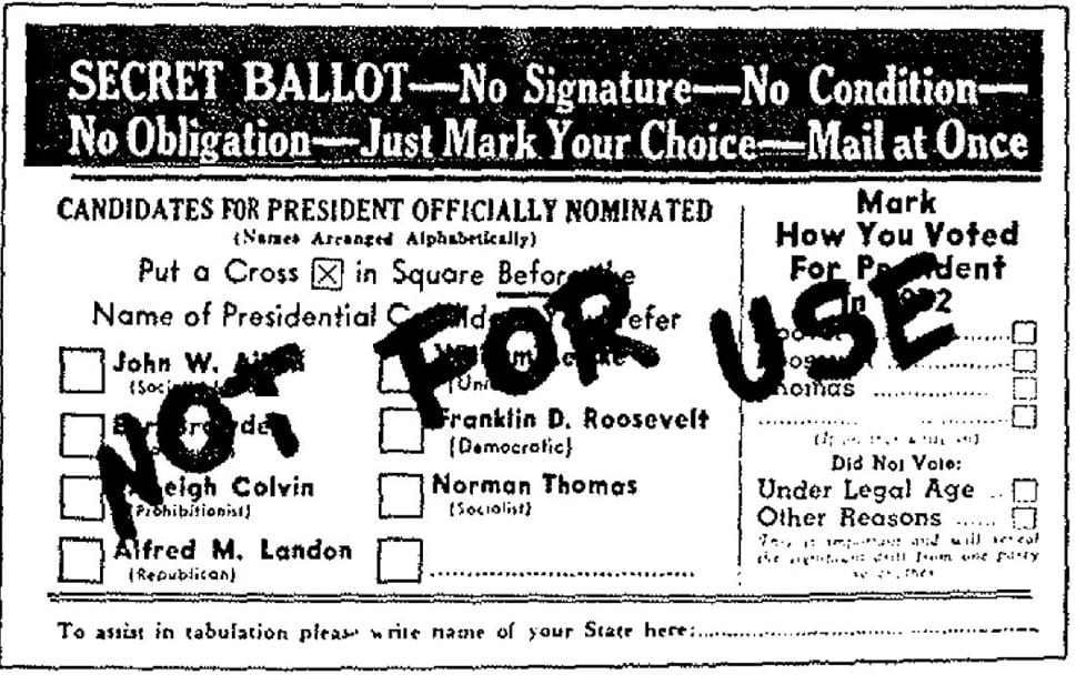
Demographic weighting could not have been used for the 1936 LD poll because those data were not collected from the respondents. But the ballot [see above] did ask respondents for whom they voted in the 1932 election. This information could have been used to weight the data using techniques that were known at that time and involved simple computations. . . .
And here’s what Lohr and Brick found:
If information collected by the poll about votes cast in 1932 had been used to weight the results, the poll would have predicted a majority of electoral votes for Roosevelt in 1936, and thus would have correctly predicted the winner of the election. We explore alternative weighting methods for the 1936 poll and the models that support them. While weighting would have resulted in Roosevelt being projected as the winner, the bias in the estimates is still very large. We discuss implications of these results for today’s low-response-rate surveys and how the accuracy of the modeling might be reflected better than current practice.
This is pretty stunning! And it provides what I think is an important lesson for statistics teaching. The usual way the Literary Digest poll is used in statistics textbooks is as a warning: Use non-probability sampling, and the boogeyman will get you! That’s pretty silly, actually, given that all polls use non-probability sampling if you consider nonresponse as part of the sampling procedure, which in effect it is. I much prefer the positive message: All samples of humans are flawed, but we can do our best to adjust for those flaws, while also recognizing the imperfections of our adjustments.
that’s really cool! i remember that from my stats classic as ‘bad’ stats. know if there’s a free pdf somewhere?
do you think the weighting methods were available to people back in 1936 or were they invented after?
interesting to think about our data today and how we might not be analyzing its full effect. maybe with new techniques future statisticians will have a better understanding of us than we do now.