In June 2025 we discussed 2 flavors of calibration, including “the logit shift”. In August 2025 we took 2nd helpings of the logit shift, focusing on multinomial outcomes. In December 2025 we took 3rd helpings, focusing on multivariate outcomes. Maybe folks have had enough (I was the only person to comment on the 3rd helpings post). But G. Elliott Morris linked to the new Will Marble and Josh Clinton multivariate logit-shifting paper, which reminded me to think about it again.

They consider the 2022 midterms in Michigan:
- y_1 = governor vote choice
- y_2 = abortion proposition vote choice
- x = demographics
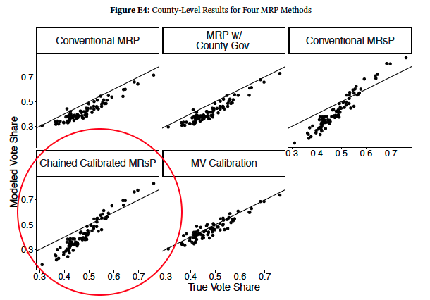
They estimate E(y_2 | county) and compare it to known truth. They have y_1, y_2, x in a survey, x in the population, and E(y_1 | county). Will and Josh look at a few estimation methods, including “Chained Calibrated MrsP“:
- Add y_1 to the population data: fit p(y_1 | x) from the survey, logit-shift to E(y_1 | county).
- MRP: fit p(y_2 | y_1, x) from the survey, average over the population distribution of y_1, x
Kuriwaki et al. 2024 do this, as we discussed in June 2025. Our mystery from December 2025 was why this method seems to do poorly in Will and Josh‘s paper:
Will suspected it was due to Jensen’s inequality, so I wrote a silly simulation to try to understand that.
n_county <- 50
n_per <- 500
b <- 8
a_county <- rnorm(n_county, -3, 2.5)
p <- runif(n_county, 0.3, 0.7)
county <- rep(1:n_county, each = n_per)
y1 <- rbinom(n_county * n_per, 1, p[county])

true_E <- tapply(seq_along(y1), county, function(ix)
mean(plogis(a_county[county[ix[1]]] +b*y1[ix])))

jensen_ignored <- plogis(a_county + b * tapply(y1, county, mean))

plot(true_E, jensen_ignored,
     xlab="True E[logit^-1(a + b*y1) | county]",
     ylab="logit^-1(a + b*E[y1|county])",
     pch=16,xlim=c(0,1),ylim=c(0,1))
abline(0, 1, col = "red", lwd = 2)

Thoughts ? Have you had enough of the logit-shift ?
Thanks Shira for the continued interest and the simulation!
Just to further explain for other readers. In the second-step of MRP — i.e. estimating y2 with y1 and x as predictors — we need the joint distribution p(y1, x). We estimate this joint distribution in the first step of MRP, in which we estimate p(y1 | x) and then use the known p(x) to obtain p(y1, x). Because we estimate p(y1 | x) with error [even after calibrating to known ground-truth margins], there is uncertainty in our estimated joint distribution. This is an issue because in order to obtain the target marginals of y2 [say, the distribution of y2 at the county level], we model p(y2 | y1, x) then integrate over the relevant portion of the joint distribution of p(y1, x). The “chained calibrated MRsP” approach uses a plug-in estimator of p(y1 | x) to compute this joint distribution, essentially treating it as if it were known without error.
My intuition was this could bias inferences due to nonlinearities in p(y1 | x). The simulation in this post look qualitatively similar to what we found in the validation exercise of our paper — suggesting I might have been on the right track. A great example of Andrew’s maxim to always do little simulations to investigate your hunches.
Btw for anyone following: I wrote an R package that implements the calibration methods in our paper. It also has some helper functions that should be useful for anyone doing MRP. Bug reports are very welcome: github.com/wpmarble/calibratedMRP
Thanks, Will ! This is super helpful.
As you say, the true E(y2 | county) = E(logit^-1(a_county + b y1) | county), an integration over y1 within county. (My little simulation dropped x.)
p(y1 | county) can be expressed with population sizes as in Kuriwaki et al. 2024 equation (3):
N_county,0/N_county * logit^-1(a_county) + N_county,1/N_county * logit^-1(a_county + b)
This is a plug-in that doesn’t propagate uncertainty in N_county,0 and N_county,1 (I’m not sure if Kuriwaki et al. talk about that ?). But it does avoid the Jensen’s inequality issue of plugging these in within the logit^-1.
Does this sound right or am I missing your point ?
Need to think more about this overall problem, but it does seem like the chained method suffers for not accounting for uncertainty around E[Y1 | X]. Presumably if you had draws from (a calibrated) p(Y1 | X) and multiply-imputed Y1, then the 2nd-stage MRP would be well-calibrated.
Thanks, Cory ! Not sure if you’re familiar with Kuriwaki et al. 2024 but can you tell if they address this uncertainty ?