Olle Folke writes:

I wanted to highlight a paper by an author who has previously been featured on your blog when he was one of the co-authors of a paper on the effect of strip clubs on sex crimes in New York. This paper looks at the effect of criminalizing the buying of sex in Sweden and finds a 40-60% increase. However, the paper is equally problematic as the one on strip clubs. In what I view as his two main specifications he using the timing of the ban to estimate the effect. However, while there is no variation across regions he uses regional data to estimate the effect, which of course does not make any sense. Not surprisingly there is no adjustment for the dependence of the error term across observations.

What makes this analysis particularly weird is that there actually is no shift in the outcome if we use national data (see figure below). So basically the results must have been manufactured. As the author has not posted any replication files it is not possible to figure out what he has done to achieve the huge increase.

I think that his response to this critique is that he has three alternative estimation methods. However, these are not very convincing and my suspicion is that neither those results would hold up for scrutiny. Also, I find the use of alternative methods both strange and problematic. First, it suggests that neither method is convincing it itself. However, doing four additional problematic analysis does not make the first one better. Also, it gives author an out when they are criticized as it involves a lot of labor to work through each analysis (especially when there is not replication data).

I took a look at the linked paper, and . . . yeah, I’m skeptical. The article begins:

This paper leverages the timing of a ban on the purchase of sex to assess its impact on rape offenses. Relying on Swedish high-frequency data from 1997 to 2014, I find that the ban increases the number of rapes by around 44–62%.

But the above graph, supplied by Folke, does not show any apparent effect at all. The linked paper has a similar graph using monthly data that also shows
nothing special going on at 1999:

This one’s a bit harder to read because of the two axes, the log scale, and the shorter time frame, but the numbers seem similar. In the time period under study, the red curve is around 5.0 on the log scale per month, 12*log(5) = 1781, and the annual curve is around 2000, so that seems to line up.

So, not much going on in the aggregate. But then the paper says:

Several pieces of evidence find that rape more than doubled after the introduction of the ban. First, Table 1 finds that the average before the ban is around 6 rapes per region and month, while after the introduction is roughly 12. Second, Table 2 presents the results of the naive analysis of regressing rape on a binary variable taking value 0 before the ban and 1 after, controlling for year, month, and region fixed effects. Results show that the post ban period is associated with an increase of around 100% of cases of rape in logs and 125% of cases of rape in the inverse hyperbolic sine transformation (IHS, hereafter). Third, a simple descriptive exercise –plotting rape normalized before the ban around zero by removing pre-treatment fixed effects– encounters that rape boosted around 110% during the sample period (Fig. 4).

OK, the averages don’t really tell us anything much at all: they’re looking at data from 1997-2014, the policy change happened in 1999, in the midst of a slow increase, and most of the change happened after 2004, as is clearly shown in Folke’s graph. So Table 1 and Table 2 are pretty much irrelevant.

But what about Figure 4:

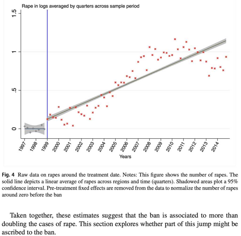
This looks pretty compelling, no?

I dunno. The first thing is that the claim that of “more than doubling” relies very strongly on the data after 2004. log(2) = 0.69, and if you look at that graph, the points only reach 0.69 around 2007, so the inference is leaning very heavily on the model by which the treatment causes a steady annual increase, rather than a short-term change in level at the time of the treatment. The other issue is the data before 1999, which in this graph are flat but in the two graphs shown earlier in this post showed an increasing trend. That makes a big difference in Figure 4! Replace that flat line pre-1999 with a positively-sloped line, and the story looks much different. Indeed, that line is soooo flat and right on zero, that I wonder if this is an artifact of the statistical fitting procedure (“Pre-treatment fixed effects are removed from the data to normalize the number of rapes around zero before the ban.”). I’m not really sure. The point is that something went wrong.

They next show their regression discontinuity model, which fits a change in level rather than slope:

There’s something else strange going on here: if they’re really fitting fixed effects for years, how can they possibly estimate a change over time? This is not making a lot of sense.

I’m not going to go through all of this paper in detail, I just did the above quick checks in order to get a rough sense what was going on, and to make sure I didn’t see anything immediately wrong with Folke’s basic analysis.

Folke continued:

The paper is even stranger than I have expected. I have gotten part of the regression code and he is estimating models that would not get any estimates on the treatment of there where no coding error (treatment is constant within years but he includes year fixed effects). Also, when I do the RDanalysis he claims he is doing I get the figure below in which there clearly is not a jump of 0.6 log points…

What the hell????

This one goes into the regression discontinuity hall of fame.

The next day, Folke followed up:

It took some digging and coding the figure out how the author was able to find such a large effect. We [Joop Adema, Olle Folke, and Johanna Rickne] have now written up a draft of a comment where we show that it is all based on a specification error and he ends up estimating something entirely different than he claims to be.

The big picture, or, how can this sort of error be avoided or its consequences mitigated

Look, everybody makes mistakes. Statistical models are hard to fit and interpret, data can be a mess, and social science theories are vague enough that if you’re not careful you can explain just about anything.

Still, it looks like this paper was an absolute disaster and a bit of an embarrassment for the Journal of Population Economics, which published it.

Should the problems been noticed earlier? I’d argue yes.

The problems with the regression discontinuity model—OK, we’re not gonna expect the author, reviewers, or editors of a paper to look too carefully at that—it’s a big ugly equation, after all—and we can’t expect author, reviewers, or editors to check the code—that’s a lot of work, right? Equations that don’t make sense, that’s just the cost of doing business.

The clear problem is the pattern in the aggregate data, the national time series that shows no jump in 1999.

I’m not saying that, just cos there’s no jump in 1999, that the policy had no effect. I’m just saying that the lack of jump in 1999 is right there for everyone to see. At the very least, if you’re gonna claim you found an effect, you’re under the scientific obligation to explain how you found that effect given the lack of pattern in the aggregate data. Such things can happen—you can have an effect that happens to be canceled out in the data by some other pattern at the same time—but then you should explain it, give that trail of breadcrumbs.

So, I’m not saying the author, reviewers, and editors of that paper should’ve seen all or even most of the problems with this paper. What I am saying is that they should’ve engaged with the contradiction between their claims and what was shown by the simple time series. To have not done this is a form of “scientism,” a kind of mystical belief in the output of a black box, a “believe the stats, not your lying eyes” kind of attitude.

Also, as Folke points out, the author of this paper has a track record of extracting dramatic findings using questionable data analysis.

I have no reason to think that the author is doing things wrong on purpose. Statistics is hard! The author’s key mistakes in these two papers have been:

1. Following a workflow in which contrary indications were ignored or set aside rather than directly addressed.

2. A lack of openness to the possibility that the work could be fatally flawed.

3. Various technical errors, including insufficient concern about data quality, a misunderstanding of regression discontinuity checks, and an inappropriate faith in robustness checks.

In this case, Adema, Folke, and Rickne did a lot of work to track down what went wrong in that published analysis. A lot of work for an obscure paper in a minor journal. But the result is a useful general lesson, which is why I’m sharing the story here.