Art Owen writes:
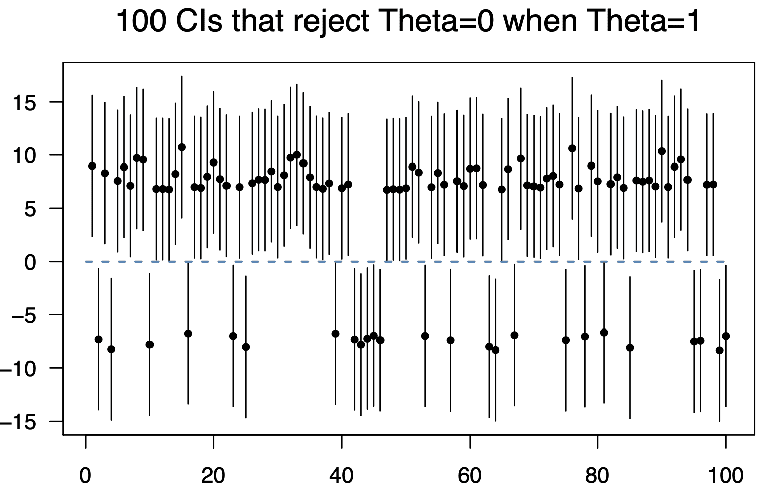
Here’s a figure you might like. I generated a bunch of data sets constructed to have true effect size 1 and power equal to 0.06. The first 100 confidence intervals that exclude 0 are shown. Their endpoints come close to the origin and their centers have absolute value far from 1. Just over 1/4 of them have the wrong sign.
When the CI endpoint is a full CI width away from zero, then you’d be pretty safe regarding the sign. Details are in this article.
I do like the above figure. It’s a very vivid expression of This is what “power = .06” looks like. Get used to it. Somebody should send it to the University of Chicago economics department.
A thought I had the other day in the context of post-hoc power analysis — since the p-value is itself a realization of some random variable (P ∈ (0,1)), can we quantify our sensitivity to significance thresholding and assess whether our observed p < alpha is itself significant at some alpha_p? As in, we observe p = 0.049, and think, oh boy, lucky me, Nature / Cell / Science here I come… but can we perform a 1-tailed test to estimate Pr(P 0.05 at alpha_p. Or maybe we can also perform a power calculation with the estimated values and see how those quantities relate?
Conversely, can we derive a probability that a given parameter estimate (from reasonable priors) is a type-M or type-S error at some degree of thresholding solely from an estimated test statistic and standard error? It’s easy to calculate these knowing the true parameter values, but what about working backwards from estimated values? Also, there’s no word for errors corresponding to appropriately signed underestimates of the magnitude of an effect, is there? For true effect, Type-S covers everything in (0, -Inf * sign(a)), type-M everything in (a, Inf * sign(a)), but what about a type… U for (0, a)? Which would correspond to errors of the sort where a p-value is high, and therefore the estimated effect size is smaller than the true effect (maybe leading researchers to conclude that a lack of significance corresponds to a lack of effect in “underpowered” studies).
Will try to give these questions some thought after a bit more coffee, but otherwise wanted to pose them here and see if y’all had any leads.
oh weird, apparently lazy guillemets trigger some fake-hyperlink markup thing? That was supposed to be an «a» after the “true effect”.
Leads? yeah sure… I’ll just check with the boys down at the stats lab. They got, uh, four more statisticians working on the case! They got us working in shifts! …. Leads *chuckles*…
There should be an uncertainty around most probabilities, because they are approximations/estimates.
In simple cases you can directly calculate the probability. Eg, after n = 3 fair coin flips there are T = 8 possible sequences: hhh, hht, hth, htt, thh, tht, tth, ttt
And there are x = 2 ways of getting all the same result. Thus the probability p of getting either all heads or tails is 2/8 = 0.25. There is no uncertainty about this value. But what if instead of d = 2 possible outcomes each trial, d can be arbitrarily large. And rather than n = 3 trials, n can be arbitrarily large. At some point, even with modern computers, you cannot directly count all the possibile configurations.
But what we can do is measure the frequency at which various outcomes occur. Back to the three coinflips, we can easily do the experiment N = 10 times. Or do a (rather verbose for clarity) simulation:
set.seed(1234)
# Do three coinflips and record results. Repeat this 10 times.
dat = replicate(10, sample(c(“H”, “T”), 3, replace = T))
# Count number of heads in each set of three flips
res = apply(dat, 2, function(x) sum(x == “H”))
# Calculate the percentage of sets that were all heads or all tails.
sum(res == 3 | res == 0)/length(res)
In that case we ger either hhh or ttt with frequency of 6 out of 10 trials. Call this proportion p_f = 0.6. But we know the actual probability is p = 0.25. So immediately we see that estimating the probability p from p_f can yield misleading results.
In the more complicated cases, we do not, and often cannot, know p. We can only know p_f. Then we try to figure out what determines the accuracy of p_f. Eg, by trying bigger and bigger numbers of replications N, we see that the value of p_f approaches our known answer of p = 0.25. Thus we learn our uncertainty about p should be inversely related to N. And so on.
I didn’t get to working out your original “alpha_p” question, but that is why what you propose would work in principle.
“When the CI endpoint is a full CI width away from zero, then you’d be pretty safe regarding the sign”
Can I just interpret that as “do NHST with alpha=4e-9?”
Assuming they were using 95% intervals, a CI width is ~4 SE, and the lower bound is ~2SE below the estimate, so I think that’s saying only estimates of ~6SE away from 0 tend to have the right sign.
ci_width <- qnorm(.975) – qnorm(.025)
est <- ci_width + qnorm(.975)
2*(1-pnorm(est))
Dan:
In the linked preprint, it says on p.5: “Suppose next, that we only declare the sign of theta to match that of theta-hat when the center theta-hat of the confidence interval is at least 2 x 1.96s away from 0.” When the estimate is 4 standard errors away from zero, the (two-sided) p-value is “only” 2*pnorm(-4)=0.00006.
Of course, this all goes out the window if there is any systematic error (bias) associated with the estimate.
This kind of plot shows up in real psycholinguistics data quite often. People‘s reaction: just count the proportion of times 0 was excluded (and presumably the sign is right). If there is a high proportion then declare that the effect is present. What does it matter that the effect is 1 or 50? Lol
Several visualizations of low power implications are shown at https://bit.ly/CH2022Kohavi slides 21-27.
In slide 18 of this talk I gave this week: https://bit.ly/ABTestsRKConvEx23, I enlarged Gelman and Carlin’s (2014) graph of the exaggeration effect, and made it much more explicit that the exaggeration goes to infinity at power = 0.05 (because that’s your type-I error rate for the null).
Power=0.06 is extremely small.