Brian Ward, Bob Carpenter, and David Barmherzig write:

The HoloML technique is an approach to solving a specific kind of inverse problem inherent to imaging nanoscale specimens using X-ray diffraction.

To solve this problem in Stan, we first write down the forward scientific model given by Barmherzig and Sun, including the Poisson photon distribution and censored data inherent to the physical problem, and then find a solution via penalized maximum likelihood. . . .

The idealized version of HCDI is formulated as
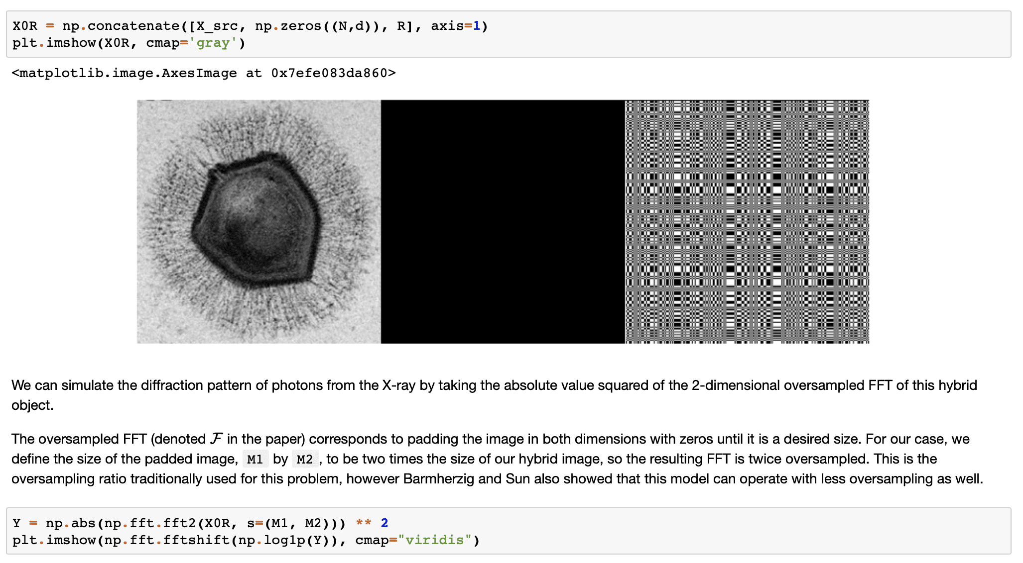
Given a reference R, data Y = |F(X+R)|^2
Recover the source image X
Where F is an oversampled Fourier transform operator.

However, the real-world set up of these experiments introduces two additional difficulties. Data is measured from a limited number of photons, where the number of photons received by each detector is modeled as Poisson distributed with expectation given by Y_ij (referred to in the paper as Poisson-shot noise). The expected number of photons each detector receives is denoted N_p. We typically have N_p < 10 due to the damage that radiation causes the biomolecule under observation. Secondly, to prevent damage to the detectors, the lowest frequencies are removed by a beamstop, which censors low-frequency observations.

In this Python notebook, Ward et al. do it all. They simulate fake data from the model, they define helper functions for their Fourier transforms in Stan (making use of Stan’s fast Fourier transform function), they write the Bayesian model (including an informative prior distribution) directly as a Stan program, they run it from Python using cmdstanpy, then they do some experimentation to see what happens when they vary the sample size of the data. The version in the case study uses optimization, but the authors tell me that sampling also works, and they’re now working on the next step, which is comparison with other methods.

I wish this computational infrastructure had existed back when I was working on my Ph.D. thesis. It would’ve made my life so much simpler—I wouldn’t’ve had to write hundreds of lines of Fortran code!

In all seriousness, this is wonderful, from beginning to end, showing how Bayesian inference and Stan can take on and solve a hard problem—imaging with less than 10 photons per detector, just imagine that!

Also impressive to me is how mundane and brute-force this all is. It’s just step by step: write down the model, program it up, simulate fake data, check that it all makes sense, all in a single Python script. Not all these steps are easy—for this particular problem you need to know a bit of Fourier analysis—but they’re all direct. I love this sort of example where the core message is not that you need to be clever, but that you just need to keep your eye on the ball, and with no embarrassment about the use of a prior distribution. This is where I want Bayesian inference to be. So thanks, Brian, Bob, and David for sharing this with all of us.

P.S. Also this, which team Google might be wise to emulate:

Reproducibility

This notebook’s source and related materials are available at https://github.com/WardBrian/holoml-in-stan.

The following versions were used to produce this page:

%load_ext watermark
%watermark -n -u -v -iv -w
print("CmdStan:", cmdstanpy.utils.cmdstan_version())

Last updated: Fri Jul 01 2022

Python implementation: CPython
Python version       : 3.10.4
IPython version      : 8.4.0

scipy     : 1.8.0
cmdstanpy : 1.0.1
numpy     : 1.22.3
IPython   : 8.4.0
matplotlib: 3.5.2

Watermark: 2.3.1

CmdStan: (2, 30)
The rendered HTML output is produced with
jupyter nbconvert --to html "HoloML in Stan.ipynb" --template classic --TagRemovePreprocessor.remove_input_tags=hide-code -CSSHTMLHeaderPreprocessor.style=tango --execute