Another example to trick Bayesian inference

This post is by Yuling, not Andrew.

We have been talking about how Bayesian inference can be flawed. Particularly, we have argued that discrete model comparison and model averaging using marginal likelihood can often go wrong, unless you have a strong assumption on the model being correct, except models are never correct. The contrast between “discrete Bayesian model comparison kinda does not work” and “Bayesian inference is the only coherent inference paradigm” bothers me. Indeed, similar counterexamples that trick discrete Bayesian model comparison can also trick discrete/continuous Bayesian inference.

Consider a toy example. We are making inferences on the location parameter in a normal model y~ normal (mu, 1) with one observation y=0. We have a restricted parameter space that only contains four points: mu belongs to {-1, 0, 1, 3}. We pose a uniform prior on mu. The inference on mu is ok: the posterior probabilities of these four points are (.27, .45, .27, .005). It is not perfect but we can interpret it as a discrete approximation to the more desired posterior in the continuous model. So far so good.

But now I want to compromise my inference. So I expand the parameter space: mu belongs to {-1, 0, 1, 3.0000, 3.0001, 3.0002, … 3.1000}; some 1000 points are inserted between 3 and 3.1. Now I still use a flat prior and make the inference. The inference is “wrong”: the posterior of mu is concentrated at 3. Indeed, the Bayesian estimate is much worse than the MLE, mu=0.

You may say it is the fault of the non-informative prior. But a naive informative prior, such as target += normal_lpdf (mu | 0, 1) still does not solve the problem. The prior needs to adjust for both the height and the volume, or what Mackay would call the Occam factor.

You may say it is the fault of the discrete parameter space, and we cannot fit this discrete model in Stan anyway. But no, similar problems can exist in continuous models. Consider the model y=0 ~ norma (mu, sigma) with a slightly constrained parameter space: |mu|<10, sigma < |mu|+1, and a flat prior on this constrained parameter space. Then the posterior inference of mu peaks at 10 or -10, which is again worse than the MLE, mu=0. Further, when changing sigma < |mu|+1 to sigma < |mu|^2+1, or to sigma < exp(|mu|)+1, the posterior will change greatly even though all priors amount to some effectively flat prior around the parameter values that we care about. Adding an extra informative prior regularization target += normal_lpdf (mu | 0, 1) solves part of the problem, but the bias from this artificially designed parameter space still carries.

The point is that the parameter space and its measure are silent subjective decisions designed by the modeler. We typically work with the counting measure on discrete space or the euclidean space with the boreal measure by default, but such assumption is context-dependent, and may be potentially falsified in a larger workflow—The Bayes rule won’t do it for you automatically.

P.S. These two examples are both artificial and is easy to fix. But the general pattern can exist in more practical examples. As Andrew pointed out in the comment, we can model the degree of freedom in a student-t likelihood as a parameter, or we may reparameterize the model into (nu, sigma*nu/(nu-2)) such that the df becomes a transformed parameter. Similarly, when modeling covariance matrix, we can model each element of the covariance matrix, model the matrix square root of it, the correlation times the diagonal, the matrix square root of the correlation times the diagonal, or the Cholesky decomposition of the correlation… Reparameterization changes the default prior and changes the “distance” between parameter values—But there are always other potential parameterizations even if we do not perform them.

Andrew pointed out two future directions. One is that we can rescue discrete model companions by designing better priors on models: to place smaller priors on similar models. I think the “dilution prior” has done that. It is related to “understanding prior in the likelihood”, and also related to the Jefferys prior that keeps the reparameterization invariant, although the latter is not always desired on other occasions.

I should also make it clear that the examples I have here can be categorized into “model misspecification”. Well, they are correct models in the classical sense: one parameter is the true value, such that with infinitely many data, everything works fine. But these models are also clearly poorly designed and a standard posterior predictive check (PPC) will manifest the poor fit.

Estimating excess mortality in rural Bangladesh from surveys and MRP

(This post is by Yuling, not by/reviewed by Andrew)

Recently I (Yuling) have contributed to a public heath project with many great collaborates: The goal is to understand the excess mortality in potential relevance to Covid-19. Before recent case surge in south Asia, we have seen stories claiming that the pandemic might have hit some low-income countries less heavily than in the US or Europe, but many low-income countries were also lacking reliable official statistics such that the confirmed Covid-19 death counts might be questionable.  To figure out how mortality changed in rural Bangladesh in 2020, my collaborates conducted repeated phone surveys in 135 villages near Dhaka, and collected death counts from Jan 2019 to Oct 2020 (the survey questions include “Was member X in your household deceased during some time range Y? When? What reason?”).

The findings

The statistical analysis appears to be straightforward: compute the mortality rate in 2019 and 2020 in the sample, subtract, obtain their difference, run a t-test, done: You don’t need a statistician. Well, not really. Some deaths were duplicately reported from multiple families, which needs preprocessing and manual inspection; the survey population dynamically changed overtime because of possible migration, newborns, deaths, and survey drop-out, so we need some survival analysis; The survey has large sample size but we also want to stratify across demographical features such as age, gender and education;  The repeated survey is not random so we need to worry about selection bias from non-response and drop-out.

It is interesting to compare these data to the birthday model on the day-of-month-effect effect. We used to make fun of meaningless heatmap comparison of day times month of birth dates. But this time the day-of-month-effect is real: participants were more likely to report death dates of deceased family members in the first half of the month as well as on some integer days.  Presumable I can model these “rounding errors” by a Gaussian process regression too, but I did not bother and simply aggregated death counts into months.

In the actual statistical modeling,  we stratify observed date into cells defined by the interaction of age, gender, month and education, and fit a multilevel logistic model: the education is not likely to have a big impact on mortality rate, but we would like to include it to adjust for non-response or drop-out bias. We poststratify the inferred mortality rate to the population and make comparison between 2019 and 2020.  The following graph shows the baseline age and month “effect”—not really causal effect though.

All coefficients are in the scale of monthly death log odd ratios. For interpretation, we cannot apply the “divide-by-four” rule as the monthly death rate is low. But because of this low rate, log odds  is close to log probability hence we can directly take exponential of a small coefficient and treat that as a multiplicative factor, which further is approximated by exp(a)-1=a. Hence a logistics coefficient of 0.1 is approximately 10% multiplicatively increase in monthly death probability (it is like “divide-by-one”,  except the genuine divide-by-four rule is on the additive probability scale).

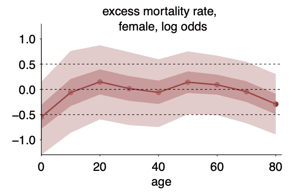
One extra modeling piece is that we want to understand the excess mortality in finer granularity. So I also model this extra risk after Feb 2020 by another multilevel regression across age, gender and education. The following graph shows the excess mortality rate by age in females and from low-education families:

This type of modeling is natural or even default to anyone familiar with this blog. Yet what I want to discuss is two additional challenges in communication.

How do we communicate excess mortality?

The figure above shows the excess mortality in terms of log odds, which in this context is close to log probability. We may want to aggregate this log odds into monthly death probability. That is done by the post-stratification step: we simulate the before and after monthly death probability for all cells, and aggregate them by 2019 census weights (in accordance to age, gender and education) in the same area. Below is the resulted excess mortality, where the unit is death count per month,

We actually see a decline in mortality starting from Feb 2020, especially for high ages (80 and above), likely due to extra cautions or family companions. Because of their high baseline values, this high age group largely dominates the overall mortality comparison. Indeed we estimate a negative overall excess mortality in this area since Feb 2020.  On the other hand, if we look into the average log odds change, the estimate is less constrained and largely overlaps with zero.

We report both results in a transparent way. You can play with our Stan code and data too. But my point here is more about how we communicate “excess mortality”. Think about an artificial make-up example: Say there are three age group, children, adults (age <59.5), elderly adults (age >59.5). Suppose they have a baseline mortality rate (0.5, 5, 30) per year per thousand people, and also assume the census proportion of these three age groups is (20%, 60%, 20%). If their mortality changes by -10%, -10%, 20%, the average percentage change is -4%.  But the absolute mortality change from (0.5, 5, 30) * (20%, 60%, 20%)=9.1 to 9.99, which is 0.89 excess death per year per thousand people, or a 0.89/9.1=10%  increase.  Is it a 10% increase, or a 4% decrease? That all depends on your interpretation. I don’t want to call it a Simpson’s paradox. Here both numbers are meaningful on its own: the average excess log mortality measures the average individual risk change;  the average excess mortality is related to death tolls. I think WHO and CDC report the latter number, but it also has the limitation of being driven by only one subgroup—we have discussed similar math problems in the context of simulated tempering and thermodynamics, and a similar story in age-adjustment over time.

The excess morality depends on the what comparison window to pick

Lastly,  the question we would like to address from the evidence of “excess morality” is essentially a causal question: what we care is the difference in death tolls if covid had not occurred hypothetically.  Except this causal question is even harder: we do not know when covid was likely to be a significant factor in this area. In other words, the treatment label is unobserved.

Instead of doing a change-point-detection, which I think would lead to non-indetfication if I would model the individual treatment effect,  I view the starting month of the excess morality comparison window as part of the causal assumption.  I fit the model with varying assumption and compute the excess mortality rate starting from Feb to Aug.   The results are interesting: the overall excess mortality is nearly negative when we compare  2020 and 2019, which is the result we report in the title. But if we choose a only compare later months, such as starting from July, there is a gradually positive excess mortality, especially for people in the age group 50–79. Well, it is not significant, and we need multiple testing when we vary these assumptions, but I don’t think a hypothesis testing is relevant here. Overall, this increasing trend is concerning, amid a more serious third wave recently in South Asia at large.

We also report the relative changes (there is always a degree of freedom to choose between multiplicative and additive effect in causal inference).

This type of varying-causal-assumption-as-much-as-you-can is what we recommend in workflow: when we have multiple plausible causal assumptions, report fits from all models (Fig 22 of the workflow paper).

But this graph leads to further questions. Recall the birthday model: if the there are fewer newborns in Halloween, then there have to be more on the days before or after. The same baby-has-to-go-somewhere logic applies here. Despite the overall excess mortality was likely negative starting from Feb 2020, we infer there was an increasing trend of mortality since the second half of 2020, especially for the age group 50–79. What we do not know for sure is whether, this positive excess mortality was a real temporal effect (a signal of gradual Covid infections), or a compensation for fewer deaths in the first half the year. Likewise, in many counties where there was a strong positive excess mortality in 2020, there could as well be a mortality decline in the following short term.  In the latter case, is this base-population change from the previous period (aka “dry tinder effect”, or the opposite wet tinder) part of the indirect effect, or mediation, of Covid-19? Or is it the confounder that we want to adjust for by fixing a constant population? The answer depends on how the “treatment” is defined, as akin to the ambiguity of a “race effect” in social science study.

size of bubbles in a bubble chart

(This post is by Yuling, not Andrew.)

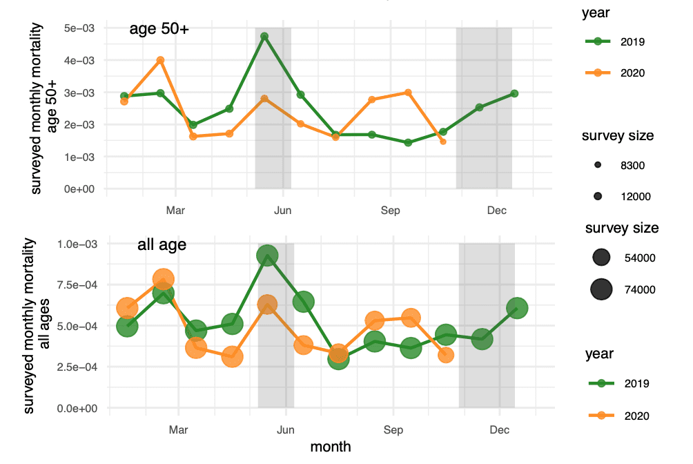
We like bubble charts. In particular, it is the go-to visualization template for binary outcomes (voting, election turnout, mortality…): stratify observations into groups, draw a scatter plot of proportions versus group feature, and use the bubble size to communicate the “group size”. To be concrete, below is a graph I draw in a recent paper, where we have survey data of mortality in some rural villages. The x-axis is the month and the y-axis the survey mortality rate that month. The size of the bubble is the accessible population size under risk during that month. I also put the older population in a separate row as their mortality rates are orders of magnitude higher.

When we make a graph comparison we always have a statistical model in mind: the scale (probability, log probability, log odds…) implies the default modeling scale; one standard error bar corresponds to a normal assumption, etc. Here, as you can imagine, we have a hierarchical model in mind and would like to partial-pool across bubbles. Visualizing the size of the bubbles implicitly conveys the message that “I have many groups! they have imbalanced group sizes! so I need a Bayesian model to enhance my small area estimation!”

OK, nothing new so far. What I want to blog about is which “group size” we should visualize. To be specific in this mortality survey, should the size be the size of the population (n), or the number of death cases (y)? I only need one of them because the y-axis indicates their ratio y/n. This distinction is especially clear for across-age comparisons.

It is common to pick to population size, which is what I did in the graph above. I also googled “gelman bubble chart election”, the first result  jumping out is the “Deep Interactions with MRP” paper in which the example visualized the subgroup population size (n) of income × ethnicity × state group, not their one-party vote count.

But I can provide a counterargument for visualizing the case size (y). Again, a graph is an implicit model: visualizing the proportion corresponds to a Bernoulli trial. The inverse Fisher information of theta in a Bernoulli (theta) likelihood is theta(1-theta). But that could be wrong unit to look at because theta is close to zero anyway. If we look at the log odds, the Fisher information of logit(theta) is theta(1-theta). In the mortality context, theta is small. Hence the “information of logit mortality” from a size-n group will be n* theta(1-theta)≈ y, which also  implies an 1/y variance scaling. This y-dependent factor will determine how much a bubble is pooled toward the shared prior mean in a multilevel posterior.

In this sense, the routine of visualizing the group size comes from a rule-of-thumb 1/n variance scaling, which is a reasonable approximation when the group-specific precision is roughly a constant.   For a Bernoulli model, the reasoning above suggests a better bubble scale could be n*theta(1-theta) ≈ y(1-n/y), but it also sounds pedantry to compute such quantities for raw data summary.

Hmmm,any experimental measure of graphical perception will inevitably not measure what it’s intended to measure.

Hierarchical stacking, part II: Voting and model averaging

(This post is by Yuling)
Yesterday I have advertised our new preprint on hierarchical stacking. Apart from the methodology development, perhaps I could draw some of your attention to the analogy between model averaging/selection and voting systems, which is likely to be more entertaining.

  • Model selection = we have multiple models to fit the data and we choose the best candidate model.
  • Model averaging = we have multiple models to fit the data and we design a weighted average of candidate models for future predictions.
  • Local model averaging = we have multiple models to fit the data and we design a weighted average of candidate  models for future predictions, and this time model weight varies in input predictors.

For notation simplicity I will consider a two-candidate situation. The easiest voting scheme is some popular vote: every ballot will be counted. In model averaging/selection, this approach corresponds to first fitting each model individually and count the utility of each model. Here voters are data points in the observation, and they are more sophisticated than casting a binary ballot. What they vote by is a continuous number depending a pre-chosen utility function (negative pointwise L2 loss, pointwise log predictive density, etc). We could replace this training error by leave-one-out cross validated error too. The bottomline is that we will count each of the ballots and add them up to obtain either the negative mean squared error or mean log predictive densities.  For Bayesian model averaging or pseudo Bayesian model averaging, we have a proportional representation system: model 1’s weight is proportional to its total voting shares (sum of pointwise log predictive densities).  For model selection using LOO-CV, we pick the candidate with who wins the popular vote.

One implication of this proportional representation system is that  a candidate would like to take care of every voter. It is something related to the “median voter theorem” in economics, but even worse: data points vote in log scale and can be widely mad if ignored. To some extent this explains why BMA is typically polarized. Imagine in a presidential election, but instead of a binary ballot to cast, voters endorse their preferences  by two positive real numbers a and b  to two candidates, such that a+b=1. A candidate’s total vote count is the multiplication of all endorsements they receive (equivalently, the summation of log a or log b they receive). The voting result will typically be quite distinct.

By contrast, we explain in the paper (Section 3) that stacking behaves like a “winner takes all”/electoral college system. That is, we first group data points/voters into two districts. Then the winner takes all shares of a district no matter how big or small the winning margin is therein.

We provide an example in which when two models become closer and closer to each other (smaller KL divergence, higher correlation of predictions, etc), their stacking weights are more distinct and eventually approach 0 and 1 when two models are nearly identical. This dynamic would never happen in a representative voting: if two candidates are identical-twins, why shouldn’t they get the same voting share? But from the standpoint of the an oracle planner/stacking, if two candidates do function identically, why should they be both kept in the administration?


Put it in another way, observing a nationwide popular vote of  51%/49% can correspond to two stories:

  • In the first story, candidate A appeals to 51% of the population but is hated by the remaining 49%. Then both BMA and stacking will assign models with the 51%/49% weight.
  • In the second possibility, these two candidates are non-identical twins, while Candidate A is superior to Candidate B by tiny margins in all aspects, such that every voter slightly prefers Candidate A and would vote for A by probability 0.51. Then BMA assigns candidate A with weight 0.51 and B with 0.49. Fair but not ideal. What stacking does is to realize that candidate A actually makes everyone better off, so as to assign it with weigh 1 regardless of the small winning margin. I think economists may call this “Pareto improvement”.

It is disputable whether or not the popular vote is more democratic than the electoral college. One advantage of the latter approach, or stacking in our context, is that a model can simply ignore some part of date and only focus on where its expertise is.  Because of the weighting in the end, two distinct models can then collaborate. What matters is not how overall-good one single candidate is, but rather how the combination can be optimized, which implicitly encourages some individual diversity.

That said, one remedy  to improve the electoral college system is to have finer-grained election districts, which is precisely what hierarchical stacking is aimed for by assigning a local weight conditional on predictors X.  That is, we group voters according to their preferences first, such that people living in the same tribe have similar views. Then we assign each tribe a local combination of candidates as per their preference. Apparently such arrangement is too complicated for any society to adopt, but at least you could apply it to your stan models and make your data points happier.

Hierarchical stacking

(This post is by Yuling)
Gregor Pirš, Aki, Andrew, and I wrote:

Stacking is a widely used model averaging technique that yields asymptotically optimal predictions among linear averages. We show that stacking is most effective when the model predictive performance is heterogeneous in inputs, so that we can further improve the stacked mixture by a full-Bayesian hierarchical modeling. With the input-varying yet partially-pooled model weights, hierarchical stacking improves average and conditional predictions. Our Bayesian formulation includes constant-weight (complete-pooling) stacking as a special case. We generalize to incorporate discrete and continuous inputs, other structured priors, and time-series and longitudinal data. We demonstrate on several applied problems.

As per the spirit of hierarchical modeling, if some quantity could vary in the population, then it should vary. Hierarchical stacking is an approach that combines models with input-varying yet partially-pooled model weights. Besides all the points we made in the paper, I personally like our new method for two reasons:

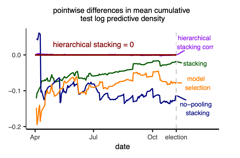
  1. We started this paper by practical motivations. Last year I was trying to use model averaging to help epidemiological predictions. Complete-pooling stacking was a viable solution, until I realized that a model good at predicting new daily cases in New York state was not necessarily good in predictions in Paris. In general, how good the model fits the data depends on what input location to condition on—All models are wrong, but some are somewhere useful. This present paper is aimed for learning where that somewhere is, and construct a local model averaging such that the model weight varies in input space. This extra flexibility comes with additional complexity, which is why we need hierarchical priors for regularization. The graph above is an example in which we average a sequence of election forecast models and allow the model weight to vary by states.
  2. In addition to this dependence on inputs, our new approach also features by its full-Bayesian formulation, whereas stacking was originally viewed as an optimization problem, or an optimization approach toward Bayesian decision problem. For some simple model like a linear regression with big n, it probably makes little difference to use MAP or MLE or average over full posterior distributions. But for complex models, this full-Bayesian approach is appealing for it
    • makes hierarchical shrinkage easier: Instead of exhaustive grid search of tuning parameters, we will be using gradient-informed MCMC;
    • provides built-in uncertainty estimation of model weights;
    • facilitates generative modeling and open-ended data inclusion: When running hierarchical stacking on election predictions, we encode prior correlations of states to further stabilize model weights in small states;
    • enables post-processing, model check, and approximate LOO-CV as if in a usual Bayesian model.

Regarding (2), we justify why this full-Bayesian inference makes sense in our formulation (via data augmentation). Looking forward, the general principle of converting a black-box learning algorithms into a generative modeling (or equivalently, a chunk of Stan code) could be a fruitful for many other methods (existing examples include KNN and SVM).  The generative model needs be specified on case-by-case basis. Take linear regression for example, the least-squares estimate of regression coefficients equivalents the MLE in a normal-error model. But we should not directly take the negative loss function as a log density and sample $latex \beta$ from $latex \log p(\beta|y)= -(x^T \beta – y)^2$+constant. The latter density  differs from the “full Bayesian inference” of the posit normal model unless $latex \sigma$ is a known constant 1. From the “marginal data augmentation” point of view, $latex \sigma$ is a working parameter that needs to be augmented in the density and avenged over in the inference—in general there could be a nuisance normalizing constant and that is when some path sampling is useful. For this additional challenge, we leave other scoring rules (interval scores, CRPS) mostly untouched in this paper, but they could be interesting to investigate, too.

This preprint is the third episode of our Bayesian model averaging series (previously we’ve had complete-pooling stacking and combining non-mixing posterior chains).

Infer well arsenic dynamic from filed kits

(This post is by Yuling, not Andrew)

Rajib Mozumder, Benjamin Bostick, Brian Mailloux, Charles Harvey, Andrew, Alexander van Geen, and I arxiv a new paper “Making the most of imprecise measurements: Changing patterns of arsenic concentrations in shallow wells of Bangladesh from laboratory and field data”. Its abstract reads:

Millions of people in Bangladesh drink well water contaminated with arsenic. Despite the severity of this heath crisis, little is known about the extent to which groundwater arsenic concentrations change over time: Are concentrations generally rising, or is arsenic being flushed out of aquifers? Are spatially patterns of high and low concentrations across wells homogenizing over time, or are these spatial gradients becoming more pronounced? To address these questions, we analyze a large set of arsenic concentrations that were sampled within a 25km2 area of Bangladesh over time. We compare two blanket survey collected in 2000–2001 and 2012–2013 from the same villages but relying on a largely different set of wells. The early set consists of 4574 accurate laboratory measurements, but the later set poses a challenge for analysis because it is composed of 8229 less accurate categorical measurements conducted in the field with a kit. We construct a Bayesian model that jointly calibrates the measurement errors, applies spatial smoothing, and describes the spatiotemporal dynamic with a diffusion-like process model. Our statistical analysis reveals that arsenic concentrations change over time and that their mean dropped from 110 to 96 μg/L over 12 years, although one quarter of individual wells are inferred to see an increase. The largest decreases occurred at the wells with locally high concentrations where the estimated Laplacian indicated that the arsenic surface was strongly concave. However, well with initially low concentrations were unlikely to be contaminated by nearby high concentration wells over a decade. We validate the model using a posterior predictive check on an external subset of laboratory measurements from the same 271 wells in the same study area available for 2000, 2014, and 2015.

For a long time, households with elevated arsenic levels have been recommended to switch to a neighbor’s safe well. Modeling the well arsenic is a familiar statistical problem that has appeared frequently in Andrew’s books and our other methodology papers. Our new paper addresses a practical question: if one switches to a tested-safe well, should they worry that the safe well may eventually be contaminated by surrounding high arsenic wells? Clearly groundwater may mix and such mixing or diffusion could eventually drive all well arsenic converge to some identical level—then why bother to switch?

To start, we worked with a small dataset containing 271 wells that were tested in 2000,2014 and 2015. If we make a linear regression of the measurements, the regression coefficient is smaller than one. Expect this is just measurement errors or regression-to-the-mean. Expect having regression-to-the-mean also does not exclude the possibility that groundwater might be actually mixing.

For the main analysis in the paper, we work with two blanket survey datasets that tested almost all wells in this area in 2000 and 2012. The statistical challenge is that (a) most wells had been reinstalled and (b) the test in 2012–2013 was conducted using field kits, which exhibited a large bias and variance.

We fit a Bayesian model that (a) calibrates this measurement error using an ordered logistic regression, (b) spatially smoothes the well arsenic surface by bivariate splines, and (c) learns the mixing dynamic.

For example if we believe the diffusion is main driving force of the arsenic mixing dynamic, we would like to estimate a diffusion equation: to regress the over-time change on Laplacian, which can be extracted from the spatial model:

Of course here we are unlikely to have a pure diffusion. We can still make some regression on Laplacian to understand the mixing dynamic. The main finding from this paper is that the largest decreases occurred at the wells with locally high concentrations where the estimated Laplacian indicated that the arsenic surface was strongly concave, while well with initially low concentrations were unlikely to be contaminated by nearby high concentration wells over a decade. This finding should be reassuring for households who rely on well-switching to reduce arsenic exposures.

Statistically, we do not invent anything new. But it does take some non-trivial efforts to combine all pieces: we know how to run spatial smoothing but now we also have biased measurements; we routinely fit differential equations in Stan but now we are dealing with a PDE on latent variables; the sample size is not very big but we have an overparameterized model (16950 free parameters) so some sparse matrices are required, etc. I am happy that some detailed statistical analysis can help solve real science problems.

The likelihood principle in model check and model evaluation

(This post is by Yuling)
The likelihood principle is often phrased as an axiom in Bayesian statistics. It applies when we are (only) interested in estimating an unknown parameter $latex \theta$, and there are two data generating experiments both involving $latex \theta$, each having observable outcomes $latex y_1$ and $latex y_2$ and likelihoods $latex p_1(y_1 \vert \theta)$ and $latex p_2(y_2 \vert \theta)$. If the outcome-experiment pair satisfies $latex p_1(y_1 \vert \theta) \propto p_2(y_2 \vert \theta)$, (viewed as a function of $latex \theta$) then these two experiments and two observations will provide the same inference information about $latex \theta$.

Consider a classic example. Someone was doing an AB testing and only interested in the treatment effect, and he told his manager that among all n=10 respondents, y=9 saw an improvement (assuming the metric is binary). It is natural to estimate the improvement probability $latex \theta$ by independent Bernoulli trial likelihood: $latex y\sim binomial (\theta\vert n=10)$. Other informative priors can exist but is not relevant to our discussion here.

What is relevant is that later the manager found out that the experiment was not done appropriately. Instead of independent data collection, the experiment was designed to sequentially keep recruiting more respondents until $latex y=9$ are positive. The actual random outcome is n, while y is fixed. So the correct model is $latex n-y\sim$ negative binomial $latex (\theta\vert y=9)$.

Luckily, the likelihood principle kicks in for the fact that binomial_lpmf $latex (y\vert n, \theta) =$ neg_binomial_lpmf $latex (n-y\vert y, \theta)$ + constant. No matter how the experiment was done, the inference remains invariant.

At the abstract level, the likelihood principle says the information of parameters can only be extracted via the likelihood, not from experiments that could have been done.

What can go wrong in model check

The likelihood is dual-purposed in Bayesian inference. For inference, it is just one component of the unnormalized density. But for model check and model evaluation, the likelihood function enables generative model to generate posterior predictions of y.

In the binomial/negative binomial example, it is fine to stop at the inference of $latex \theta$. But as long as we want to check the model, we do need to distinguish between the two possible sampling distributions and which variable (n or y) is random.

Consider we observe y=9 positive cases among n=10 trials, with the estimated $latex \theta=0.9$, the likelihood of binomial and negative binomial models are

> y=9
> n=10
> dnbinom(n-y,y,0.9)
 	 0.3486784
> dbinom(y,n, 0.9)
	0.3874205

Not really identical. But the likelihood principle does not require them to be identical. What is needed is a constant density ratio, and that is easy to verify:

> dnbinom(n-y,y, prob=seq(0.05,0.95,length.out = 100))/dbinom(y,n, prob=seq(0.05,0.95,length.out = 100))

The result is a constant ratio, 0.9.

However, the posterior predictive check (PPC) will have different p-values:

> 1-pnbinom(n-y,y, 0.9)
 	0.2639011
> 1-pbinom(y,n, 0.9)
	0.3486784

The difference of the PPC-p-value can be even more dramatic with another $latex \theta$:

> 1-pnbinom(n-y,y, 0.99)
 	0.0042662
> 1-pbinom(y,n, 0.99)
	0.9043821

Just very different!

Clearly using Bayesian posterior of $latex \theta$ does not fix the issue. The problem is that likelihood ensures some constant ratio on $latex \theta$, not on $latex y_1$ nor $latex y_2$.

Model selection?

Unlike the unnormalized likelihood in the likelihood principle, the marginal likelihood in model evaluation is required to be normalized.

In the previous AB testing example, given data $latex (y,n)$, if we know that one and only one of the binomial or the negative binomial experiment is run, we may want to make model selection based on marginal likelihood. For simplicity we consider a point estimate $latex \hat \theta=0.9$. Then we obtain a likelihood ratio test, with the ratio 0.9, slightly favoring the binomial model. Actually this marginal likelihood ratio is constant y/n, independent of the posterior distribution of $latex \theta$. If $latex y/n=0.001$, then we get a Bayes factor 1000 favoring the binomial model.

Except it is wrong. It is not sensible to compare a likelihood on y and a likelihood on n.

What can go wrong in cross-validation

CV requires some loss function, and the same predictive density does not imply the same loss (L2 loss, interval loss, etc.). For adherence, we adopt log predictive densities for now.

CV also needs some part of the data to be exchange, which depends on the sampling distribution.

On the other hand, the calculated LOO-CV of log predictive density seems to only depend on the data through the likelihood. Consider two model-data pair $latex M1: p_1(\theta\vert y_1)$ and $latex M2: p_2(\theta\vert y_2)$, we compute the LOOCV by $latex \text{LOOCV}_1= \sum_i \log \int_\theta {\frac{ p_\text{post} (\theta\vert M_1, y_1)}{ p_1(y_{1i}\vert \theta) }} \left({ \int_{\theta} { p_\text{post} (\theta\vert M_1, y_1)}{ p_1(y_{1i}\vert \theta) }d\theta}\right)^{-1} p_1 (y_{{1i}}\vert\theta) d\theta,$ and replace all 1 with 2 in $latex \text{LOOCV}_2$.

The likelihood principle does say that $latex p_\text{post} (\theta\vert M_1, y_1)=p_\text{post} (\theta\vert M_2, y_2) $, and if there is some generalized likelihood principle ensuring that $latex p_1 (y_{1i}\vert\theta)\propto p_2 (y_{2i} \vert\theta)$, then $latex \text{LOOCV}_1= \text{constant} + \text{LOOCV}_2$.

Sure, but it is an extra assumption. Arguably the point-wise likelihood principle is such a strong assumption that would hardly be useful beyond toy examples.

The basic form of the likelihood principle does not have the notation of $latex y_i$. It is possibles that $latex y_2$ and $latex y_1$ have different sample size: consider a meta-polling with many polls. Each poll is a binomial model with $latex y_i\sim binomial(n_i, \theta)$. If I have 100 polls, I have 100 data points. Alternatively I can view data from $latex \sum {n_i}$ Bernoulli trials, and the sample size becomes $latex \sum_{i=1}^{100} {n_i}$.

Finally just like the case in marginal likelihood, even if all conditions above hold, regardless of the identity, it is conceptually wrong to compare $latex \text{LOOCV}_1$ with $latex \text{LOOCV}_2$. They are scoring rules on two different spaces (probability measures on $latex y_1$ and $latex y_2$ respectively) and should not be compared directly.

PPC again

Although it is a bad practice, we sometimes compare PPC p-values from two models for the purpose of model comparison. In the y=9, n=10, $latex \hat\theta=0.99$ case, we can compute the two-sided p-value: min( Pr(y_{sim} > y), Pr(y_{sim} < y)) for the binomial model, and min( Pr(n_{sim} > n), Pr(n_{sim} < n)) for the NB model respectively.

> min(pnbinom(n-y,y, 0.99),  1-pnbinom(n-y,y, 0.99) )
  0.004717254
> min( pbinom(y,n, 0.99),   1-pbinom(y,n, 0.99))
  0.09561792

In the marginal likelihood and the log score case, we know we cannot directly compare two likelihoods or two log scores when they are on two sampling spaces. Here, the p-value is naturally normalized. Does it mean we the NB model is rejected while the binomial model passes PPC?

Still we cannot. We should not compare p-values at all.

Model evaluation on the joint space

To avoid unfair comparison of marginal likelihoods and log scores across two sampling spaces, a remedy is consider a product space: both y and n are now viewed as random variables.

The binomial/negative binomial narrative specify two joint models $latex p(n,y\vert \theta)= 1(n=n_{obs}) p(y\vert n, \theta)$ and $latex p(n,y\vert \theta)= 1(y=y_{obs}) p(n\vert y, \theta)$.

The ratio of these two densities only admit three values: 0, infinity, or a constant y/n.

If we observe several paris of $latex (n, y)$, we can easily decide which margin is fixed. The harder problem is we only observe one $latex (n,y)$. Based on the comparison of marginal likelihoods and log scores in the previous sections, it seems both metric would still prefer the binomial model (now it is viewed as a sampling distribution on the product space).

Well, it is almost correct expect that 1) the sample log score is not meaningful if there is only one observation and 2) we need some prior on models to go from marginal likelihood to the Bayes factor. After all, under either sampling model, the event admitting nontrivial density ratios, $latex 1(y=y_{obs}) 1(n=n_{obs})$, has zero measure. It is legit to do model selection/comparison on the product space, but we could do whatever we want at this point without affecting any property in almost sure sense.

Some causal inferene

In short, the convenience of inference invariance from the likelihood principle also makes it hard to practise model selection and model evaluation. The latter two modules rely on the sampling distribution besides the likelihood.

To make this blog post more confusing, I would like to draw some remote connection to causal inference.

Assuming we have data (binary treatment: z, outcome y, covariate: x) from a known model M1: y = b0 + b1 z + b2 x + iid noise. If the model is correct and if there is no other unobserved confounders, we estimate the treatment effect of z by b1.

The unconfoundedness assumption requires that y(z=0) and y(z=1) are independent of z given x. This assumption is only a description on causal interpretation, and never appears in the sampling distribution or the likelihood. Assuming there does exist a confounder c, and the true DG is M2: y | (x, z, c) = b0 + b1 z + b2 x + c + iid noise, and z | c= c + another iid noise. Then marginalize-out c (because we cannot observe it in data collection), M2 becomes y | x, z= b0 + b1 z + b2 x+ iid noise. Therefore, (M1, (x, y, z)) and (M2, (x,y,z)) admit an experiment-data pair on which the likelihood principle holds. It is precisely the otherwise lovely likelihood principle that excludes any method to test the unconfoundedness assumption.

From monthly return rate to importance sampling to path sampling to the second law of thermodynamics to metastable sampling in Stan

(This post is by Yuling, not Andrew, except many ideas are originated from Andrew.)

This post is intended to advertise our new preprint Adaptive Path Sampling in Metastable Posterior Distributions  by Collin, Aki, Andrew and me, where we developed an automated implementation of path sampling and adaptive continuous tempering. But I have been recently reading a writing book and I am convinced that an advertisement post should always start by stories to hook the audience, so let’s pretend I am starting this post from the next paragraph with an example.

Some elementary math about geometric means

To start, one day I was computing my portfolio return, but I was doing that in Excel, in which the only function I knew is mean and sum. So I would simply calculate the average monthly return, and multiply it by 12.

Of course you do not really open your 401K account now. We can simulate data in R too, which amounts to:

month_return=rnorm(60,.01,0.04)
print(mean(month_return)*12)

Sure, it is not the “annualized return”. A 50% gain followed by a 50% loss in the next month results in 1.5* 0.5 = 0.75, or a 25% loss. Jensen’s inequality ensures that the geometric mean is always smaller than the arithmetic mean.

exp(mean(log(1+ month_return)))-1- mean(month_return)

That said, this difference is small since the monthly return itself is typically close enough to zero. But even to annualize these two estimates to a whole year still yields a nearly identical annualized return value:

exp(mean(log(1+month_return)))^12-1 - mean(month_return)*12

Intuitively, the arithmetic mean is larger per unit, but is also offset by lack of the compound interest.
It is not anything surprising beyond elementary math. The first order Taylor series expansion says
$latex \log (1+ x) \approx x, $
for any small x. And the geometric mean of x is really the arithmetic mean of log (1+ x). Indeed in the limit of per second return, by integrating both sides, these two approaches are just identical. When per unit change of x is not smooth enough (i.e. too big gap), the second order term -.5 sd(x) will kick in via Itô calculus, but that is irreverent to what I will discuss next. Also the implicit assumption here is that x>-1 otherwise log(1+x) becomes invalid, so this asymptotical equivalence will also fail if the account is liquidated, but that is more irreverent to what I will discuss.

The bridge between Taylor series expansion and importance sampling

Forget about finance, let’s focus on the normalizing constant in statistical computing. In many statistical problems, including marginal likelihood computation and marginal density/moment estimation in MCMC, we are given an unnormalized density $latex q(\theta, \lambda)$, where $latex \theta \in \Theta$ is a multidimensional sampling parameter and $latex \lambda \in \Lambda$ is a free parameter, and we need to evaluate the integrals $latex z(\lambda)$=$latex \int_{\Theta} q(\theta, \lambda) d \theta$, for any $latex \lambda \in \Lambda.$

Here z(.) is a function of $latex \lambda$. For convenience let’s still call z() the normalizing constant without mentioning function.

Two accessible but conceptually orthogonal approaches stand out for the normalizing constant. Viewing it as the expectation with respect to the conditional density $latex \theta|\lambda \propto q(\theta, \lambda)$, we can numerically integrate it using quadrature, where the simplest is linearly interpolation, and first order Taylor series expansion yields
$latex \log\frac{z(\lambda)}{z(\lambda_0)}$ $latex \approx (\lambda – \lambda_0) \frac{1}{ z(\lambda_0)}\int_\Theta (\frac {d}{d \lambda }q(\theta, \lambda) | {\lambda=\lambda_0} )d \theta.$
In contrast, we can sample from the conditional density $latex \theta| \lambda_0 \propto q(\theta, \lambda_0)$, and apply importance sampling,
$latex \frac{z(\lambda)}{z(\lambda_0)}\approx\frac{1}{S}\sum_{s=1}^S$ $latex \frac{ q (\theta_s, \lambda)}{q(\theta_s, \lambda_0)}$, $latex \theta_{s=1, \cdots, S} \sim q (\theta, \lambda_0).$
Due to the same reason that the annualized arithmetic return equivalents the geometric return, the first order Taylor series expansion and importance sampling reach the same first order limit when the proposal is infinitely close to the target. That is, for any fixed $latex \lambda_0$, as $latex \delta=|\lambda_1 – \lambda_0|\to 0$,
$latex \frac{1}{\delta}\log E_{\lambda_{0}}\left[\frac{q(\theta|\lambda_{1})}{q(\theta|\lambda_0)}\right]$ = $latex \int_{\Theta} \frac{\partial}{\partial \lambda} \log q(\theta|\lambda_{0}) p(\theta|\lambda_0)d\theta + o(1)= \frac{1}{\delta}E_{\lambda_{0}}\left[ \log \frac{q(\theta|\lambda_{1})} {q(\theta|\lambda_0)}\right].$

Path sampling

The path sampling estimate is just the integral of the dominate term in the middle of the equation above:
$latex \frac{z(\lambda_1)}{z(\lambda_0)}\approx\int_{\lambda_0}^{\lambda_1}\int_{\Theta} \frac{\partial}{\partial \lambda} \log q(\theta|\lambda_{l}) p(\theta|\lambda_l)d\theta d \lambda.$
In such sense, the path sampling is the continuous limit of both the importance sampling and the Taylor expansion approach.

More generally, if we draw $latex (a, \theta)$ sample from the joint density
$latex p(a,\theta)\propto\frac{1}{c(a)}q(\theta,\lambda=f(a)),$
where $latex c()$ is any pseudo prior, and $latex a$ is a transformed parameter of lambda through a link function f(), then the thermodynamic integration (Gelman and Meng, 1998, indeed dated back to Kirkwood, 1935) yields the identity
$latex \frac{d}{da}\log z(f(a))=E_{\theta|f(a)}\Bigl[\frac{\partial}{\partial a}\log\left(q(\theta, f(a)\right)\Bigr],$
where the expectation is over the invariant conditional distribution $latex \theta | a \propto q(\theta, f(a))$.

If a is continuous, this conditional $latex \theta|f(a)$ is hard to evaluate, as typically there is only one theta for each unique $latex a$. However, it is still a valid stochastic approximation to approximate
$latex E_{\theta|f(a_i)}\Bigl[\frac{\partial}{\partial a}\log\left(q(\theta,f(a)\right)\Bigr]\approx\frac{\partial}{\partial a}\log\left(q(\theta_i, f(a_i)\right)$
by one Monte Carlo draw.

Continuously simulated tempering on an isentropic circle

Simulated tempering and its variants provide an accessible approach to sampling from a multimodal distribution. We augment the state space $latex \Theta$ with an auxiliary inverse temperature parameter $latex \lambda$, and employ a sequence of interpolating densities, typically through a power transformation $latex p_j\propto p(\theta|y)^{\lambda_j}$ on the ladder 0=$latex \lambda_0 \leq \cdots\leq \lambda_K=1$,
such that $latex p_K$ is the distribution we want to sample from and $latex p_0$ is a (proper) base distribution. At a smaller $latex \lambda$, the between-mode energy barriers in $latex p(\theta|\lambda)$ collapse and the Markov chains are easier to mix. This dynamic makes the sampler more likely to fully explore the target distribution at $latex \lambda=1$. However, it is often required to scale the number of interpolating densities K at least O(parameter dimension), soon becoming unaffordable in any moderately high dimensional problems.

A few years ago, Andrew came up with this idea to use path sampling in continuous simulated tempering (I remember he did so during one BDA class when he was teaching simulated temperimg). In this new paper, we present an automated way to conduct continuously simulated tempering and adaptive path sampling.

The basic strategy is to augment the target density $latex q(\theta)$, potentially multimodal, by a tempered path
$latex 1/c(\lambda)\psi(\theta)^{1-\lambda}q(\theta)^{\lambda}$ where $latex \psi$ is some base measurement. Here the temperature lambda is continuous in [0,1], so as to adapt to regions where the conditional density changes rapidly with the temperature (which might be missed by discrete tempering).

Directly sampling from theta and lambda makes it hard to access the samples from the target density (as Pr(lambda=1)=0 in any continuous densities). Hence we further transform theta into a transformed $latex a$ using a piecewise polynomial link function $latex \lambda=f(a)$ like this,

An $latex a$-trajectory from 0 to 2 corresponds to a complete $latex \lambda$ tour from 0 to 1 (cooling) and back down to 0 (heating). This formulation allows the sampler to cycle back and forth through the space of lambda continuously, while ensuring that some of the simulation draws (those with a between 0.8 and 1.2) are drawn from the exact target distribution with $latex \lambda=1$. The actual sampling takes place in $latex a\in [0,2]\times\theta\in\Theta$. It has a continuous density and is readily implemented in Stan.

We then use path sampling compute the log normalizing constant of this system, and adaptive modify the a-margin to ensure a complete cooling-heating cycle.

Notable, in discrete simulated tempering and annealed importance sampling, we typically compute the marginal density and the normalization constant
$latex \frac{z_{\lambda_K}}{z_{\lambda_0}}=E\left[\exp\mathcal{W}(\theta_0,\dots,\theta_{K-1})\right],\mathcal{W}(\theta_0,\dots,\theta_{K-1})=\log\prod_{j=0}^{k-1}\frac{q(\theta_j,\lambda_{j+1})}{q(\theta_j,\lambda_{j})}.$
In statistical physics, the $latex \mathcal{W}$ quantity can be interpreted as virtual work induced on the system. The same Jensen’s inequality that has appeared twice above leads to $latex E \mathcal{W} \geq \log z(\lambda_K)- \log z(\lambda_0)$. This is a microscopic analogy to the second law of thermodynamics: the sum of work entered in the system is always larger than the free energy change, unless the switching is processed infinitely slow, which corresponds to the proposed path sampling scheme where the interpolating densities are infinitely dense. A physics minded might call this procedure a reversible-adiabatic/isentropic/quasistatic process—It is the conjunction of path sampling estimation (unbiased for free energy) and the continuous tempering (infinitely many interpolating states) that  preserves the entropy.

This asymptotic equivalence between importance sampling based tempering and continuous tempering is again the same math behind the annualize return example. The log (1+ monthly return) term now corresponds the free energy (log normalization constant) difference between two adjacent temperatures, which are essentially dense in our scheme.

Practical implementation in Stan

Well, if the blog post is an ideal format for writing math equations, there would not be journal articles, the same reason that MCMC will not exist if importance sampling scales well. Details of our methods are better summarized in the paper. We also provide an easy access to continuous tempering in R and Stan for a black box implementation of path sampling based continuous tempering.
Consider the following Stan model:

data {
real y;
}
parameters {
real theta;
}
model{
y ~ cauchy(theta, 0.1);
-y ~ cauchy(theta, 0.1);
}

With a moderately large input data y, the posterior distribution of theta will be only be asymptotically changed at two points close to y and -y. As a result, Stan cannot fully sample from this two-point-spike even with a large number of iterations.

To run continuous tempering, a user can specify any base model, say normal(0,5), and list it in an alternative model block as if it is a regular model.

model{ // keep the original model
  y ~ cauchy(theta,0.1);
  -y ~ cauchy(theta,0.1);
}
alternative model{ // add a new block of the base measure (e.g., the prior).
  theta ~ normal(0,5);
}

Save this as `cauchy.stan`. To run path sampling, simply run

devtools::install_github("yao-yl/path-tempering/package/pathtemp")
library(pathtemp)
update_model <- stan_model("solve_tempering.stan")
#https://github.com/yao-yl/path-tempering/blob/master/solve_tempering.stan
file_new <- code_temperature_augment("cauchy.stan")
sampling_model <- stan_model(file_new) # compile
path_sample_fit <- path_sample(data=list(gap=10), # the data list in original model,
                               sampling_model=sampling_model,
                               N_loop=5, iter_final=6000)

The returned value provides access to the posterior draws from the target density and base density, the join path in the final adaptation, and the estimated log normalizing constant.

 sim_cauchy <- extract(path_sample_fit$fit_main)
in_target <- sim_cauchy$lambda==1
in_prior <- sim_cauchy$lambda==0
# sample from the target
hist(sim_cauchy$theta[in_target])
# sample from the base
hist(sim_cauchy$theta[in_prior])
# the joint "path"
plot(sim_cauchy$a, sim_cauchy$theta)
# the normalizing constant
plot(g_lambda(path_sample_fit$path_post_a), path_sample_fit$path_post_z)

Here is the output.

Have fun playing with code!

Let me close with two caveats. First, we don’t think tempering can solve all metastability issues in MCMC. Tempering imposes limitations on dimensions and problem scales. We provide a failure mode example where the proposed tempering scheme (or any other tempering methods) fails. Adaptive path sampling comes with an importance-sampling-theory-based diagnosis that makes this failure manifest. That said, in many cases we find this new path-sampling-adapted-continuous-tempering approach performs better than existing methods for metastable sampling. Second, posterior multimodality often betokens model misspecification (we discussed this in our previous paper on chain-stacking). The ultimate goal is not to stop at the tempered posterior simulation draws, but to use them to check and improve the model in a workflow.


How good is the Bayes posterior for prediction really?

It might not be common courtesy of this blog to make comments on a very-recently-arxiv-ed paper. But I have seen two copies of this paper entitled “how good is the Bayes posterior in deep neural networks really” left on the tray of the department printer during the past weekend, so I cannot underestimate the popularity of the work.

So, how good is the Bayes posterior in deep neural networks really, especially when it is inaccurate or bogus?

The paper argues that in a deep neural network, for prediction purposes, the full posterior yields a worse accuracy/cross-extropy than the one from the point estimation procedures such as stochastic gradient descent (sgd). Even more strikingly, it claims that a quick remedy, no matter how ad hoc it may look like, is to reshape the posterior via a power transformation, which they call a “cold posterior” $latex \propto (p(\theta|y))^{1/T}$ for temperature T<1.  Effectively the cold temperature concentrates the posterior density more around the MAP. According to the empirical evaluation the authors claim the cold posterior is superior to both the exact posterior and the point estimation in terms of predictive performance.

First of all, I should congratulate the authors for their new empirical results on Bayesian deep learning, a field that seems to have been advocated back to a few decades ago but neither sophisticatedly defended nor comprehensively applied, at least for modern-day deep models. Presumably the largest barrier is computation, as the exact sampling from a posterior in a deep net is infeasible given today’s computer.

Indeed, even in this paper, it is hard for me to tell, if the undesired performance of “exact” Bayesian posterior prediction is attributed to Thomas Bayes, or to Paul Langevin: the authors use an overdamped Langevin dynamic to sample from the posterior, except for omitting the Metropolis adjustment. They do report some diagnostics, but not quite exhaustive, as a more apparent and arguably more powerful test is to run multiple chains and see if they have mixed. Later in their section 4.4, the authors seem not to distinguish between the Monte Carlo error and the sampling error, and suggest even the first term can to too large in the method, which makes me even more curious how reliable the “posterior” is. Further, according to figure 4, there is an obvious discrepancy between the samples (over all temperatures) drawn from HMC and the Langevin dynamic used here even in a toy example with network depth to be 2 or 3. I don’t think HMC itself is necessarily the gold standard either:  In a complicated model such as ResNet, HMC suffers from all multimodality and non-log-convexity, and would hardly mix. So are we just blaming the Bayesian posterior from some points that were drawn from a theoretically-biased and practically-hardly-converged sampler?

In section 5, the authors conjecture that deep learning practice violates the likelihood principle because of some computation techniques such as dropout. To me, this is not what the likelihood principle is particularly relevant. Rather it is another reason why the posterior from the proposed sampler is computationally concerning.

To be fair, for the purpose of point estimation, even sgd is not necessarily guaranteed to either theoretically converge to, nor practically well approximate the global optimum either, while in most empirical studies it still yields reasonable predictions.  This reminds me of a relevant paragraph by Gelman and Robert (2013):

In any case, no serious scientist can be interested in bogus arguments (except, perhaps, as a teaching tool or as a way to understand how intelligent and well-informed people can make evident mistakes, as discussed in chapter 3 of Gelman et al. 2008). What is perhaps more interesting is the presumed association between Bayes and bogosity. We suspect that it is Bayesians’ openness to making assumptions that makes their work a particular target, along with (some) Bayesians’ intemperate rhetoric about optimality.

Sure, I guess it might be also unfair that we are kinda rewarding Bayes for it is more likely to produce fragile and bogus computational results. That said, the discussion here does not dismiss the value of this new paper, in which part of the merit is to alert Bayesian deep learning researchers that many otherwise fine sampler may produce inaccurate or bogus posteriors in these deep models, and all these computation errors should be taken into account for prediction evaluations.

But the intemperate rhetoric about optimality is real

The discussion below is not directly related to that paper. But an even more alarming and less understood question is, how good is the predictive performance of Bayes posterior in a general model when it is computationally accurate?  

As far as I know, Bayes procedures do not necessarily automatically improve the prediction or calibration over a point estimation such as the MAP.

I collected a few paradoxical examples when I wrote our old paper on variational inference diagnostics. Without the need for a residual net, even in a linear regression I can find examples in which exact Bayesian posterior lead to worse predictive performance than ADVI (Reproducible code is available upon request). This is not a pathological edge example. The data is simulated from the correctly-specified regression model with n=100 and d=20 — and these are exactly the data one would simulate for linear regressions. The posterior is sampled using stan and is exact measured by all diagnostics. The predictive performance is evaluated using log predictive density on independent test data and the averaged over a large number of replications of both data and sampling to eliminate all other noises. But still, log predictive density from ADVI is higher than the exact posterior.

In this experiment, I also examined that ADVI has a large discrepancy compared with the exact one, revealed by a large k hat from our psis diagnostics. So basically it is a somewhat “cold-posterior” in terms of underdispersion.

At the immediate level,  the underdispersion from variational inference can serve as an implicit prior which might render the model more regularization and therefore improve the prediction. For the record, I already encode an N(0,2) prior on all regression coefficient in that example with all unit inputs. In general, however, many complicated models used in practice lack informative priors, and it could be the reason why a stronger regularization, or via a “colder” posterior could help– although it is more suggested to come with a reasonable informative prior directly rather than tune the “temperature” for the sake of both interpretation and a coherent workflow.

Secondly, a model/regularization good for point estimation,  is not necessarily good for Bayesian posteriors. We can recall a Bayesian lasso gives inferior performance than the horseshoe, though it is often what is needed for point estimations. This is also the example in which the regularization effect from prior cannot be simplified by a temperature rescaling as the horseshoe has both thicker tail and thicker zero than Laplace prior. In that deep learning context, does the network architecture and all implicit regularizations such as dropout that were motivated from, designed for, and often cases optimally-tuned towards MAP estimates necessarily good/enough for posteriors? We do not know.

Coincidentally,  Andrew and I recently wrote a paper on Holes in Bayesian Statistics:

It is a fundamental principle of Bayesian inference that statistical procedures do not apply universally; rather, they are optimal only when averaging over the prior distribution. This implies a proof-by-contradiction sort of logic … it should be possible to deduce properties of the prior based on understanding of the range of applicability of a method.

In short, it is not too surprising that the exact Bayesian posterior can give an inferior prediction than MAP or VI, if we are merely using a black-box model and treat it as it is. But,

This does not mean that we think Bayesian inference is a bad idea, but it does mean that there is a tension between Bayesian logic and Bayesian workflow which we believe can only be resolved by considering Bayesian logic as a tool, a way of revealing inevitable misfits and incoherences in our model assumptions, rather than as an end in itself.


P.S. (from Andrew): Yuling pointed me to the above post, and I just wanted to add that, yes, I do sometimes encounter problems where the posterior mode estimate makes more sense than the full posterior. See, for example, section 3.3 of Bayesian model-building by pure thought, from 1996, which is one of my favorite articles.

As Yuling says, the full Bayes posterior is the right answer if the model is correct—but the model isn’t ever correct. So it’s an interesting general question: when is the posterior dominated by a mode-based approximation? I don’t have a great answer to this one.

Another good point made by Yuling is that “the posterior” isn’t always so clearly defined, in that, in a multimodal setting, the computed posterior is not necessarily the same as the mathematical posterior from the model. Similarly, in a multimodal distribution, “the mode” isn’t so clearly defined either. We should finish our paper on stacking for multimodal posteriors.

Lost of good question shere, all of which are worth thinking about in an open-minded way, rather than as a Bayes-is-good / Bayes-is-bad battle. We’re trying to do our part here!

“Machine Learning Under a Modern Optimization Lens” Under a Bayesian Lens

I (Yuling) read this new book Machine Learning Under a Modern Optimization Lens (by Dimitris Bertsimas and Jack Dunn) after I grabbed it from Andrew’s desk. Apparently machine learning is now such a wide-ranging area that we have to access it through some sub-manifold so as to evade dimension curse, and it is the same reason why I would like to discuss this comprehensive and clearly-structured book through a Bayesian perspective.

Regularization and robustness, and what it means for priors

The first part of the book is most focused on the interpretation of regularization and robustness (Bertsimas and Copenhaver, 2017). In a linear regression with data $latex (X,Y)$, we consider a small perturbation within the neighborhood $latex \Delta \in \mathcal{U}(q,r)= \{\Delta\in \mathcal{R}^{n\times p}: \max_{\vert\vert \delta \vert\vert_{q} =1 } \vert\vert \delta \Delta \vert\vert_{r} \},$ then the $latex l_q$ regularized regression is precisely equivalently to the minimax robustness:
$latex \displaystyle \min_{\beta}\max_{\Delta\in \mathcal{U}(q,r)} \vert\vert y-(X+\Delta)\beta \vert\vert_{r} = \min_{\beta} \vert\vert y-(X+\Delta)\beta \vert\vert_{r} + \vert\vert \beta \vert\vert_{q} $
and such equivalence can also be extended to other norms too.

The discussion of this book is mostly useful for point estimation in a linear regression. As a Bayesian, it is natural to ask, if we could also encode the robustness constraints into the prior for a general model. For example, can we establish something like (I suppress the obvious dependence on X):
$latex \displaystyle \min_{p^{post}} \max_{ p^*: D(p^* \vert\vert p^{sample})<\epsilon } – \int_{\tilde y} \log \int_{\theta} p(\tilde y \vert \theta ) p^{post}(\theta ) d\theta p^*(\tilde y\vert y ) d \tilde y= – \int_{\tilde y} \log \int_{\theta} p(\tilde y \vert \theta) p(\theta\vert y ) d\theta p^{sample}(\tilde y\vert y ) d \tilde y.
$
where is $latex p(\theta\vert y ) \propto p(\theta)p(y\vert \theta)$ is the Bayesian posterior distribution under certain prior that is potentially induced by this equation, and $latex y_{1,\dots,n}$ are iid samples from $latex p^{sample}$, which are however different from the future new samples $latex \tilde y \sim p^*(\tilde y)$ up to a $latex \epsilon$ perturbation under some divergence $latex D(\cdot|\cdot)$.

In other words, we might wish to construct the prior in such a way that the model could still give minimax optimal prediction even if the sampling distribution is slightly corrupted.

To be clear, the equivalence between a minimax (point-)estimation and the least-favorable prior is well studied. However here the minimax is the minimax out-of-sample risk of the prediction of the data, rather than the classic risk of the parameter estimation, where the only bridge is through the likelihood.

It also reminds me of our PSIS leave-one-out(LOO). In particular, we know where the model behaves bad (e.g. points with large k hat $latex >\epsilon$). It makes sense, for example, if we encode these bad points into the prior adaptively
$latex \displaystyle \log p^{prior}(\theta) \gets \log p^{prior}(\theta) + \gamma\log \sum_{i: k_{i}>\epsilon} p( y_i\vert\theta) $
and retrain the model either explicitly or through importance sampling. It is of course nothing but adversarial training in deep leaning.

Nevertheless, it is the time to rethink what a prior is aimed for:

  1. In terms of prior predictive check, we implicitly ask for a large or even the largest (in empirical Bayes) marginal likelihood $latex \int p(y\vert \theta) p(\theta) d\theta$.
  2. But prior is also just regularization, and regularization is just robustness from the previous argument. It is not because we or any other people have enough reasons to believe the regression coefficient perfectly forms a Laplace distribution that we use the Lasso; it is rather because we want our model to be more robust under some $latex l_1$ perturbation in the data. An adversarial training weighs more on “bad” data points and therefore deliberately decrease the prior predictive power, in exchange for robustness.

Let me recall Andrew’s old blog: What is the “true prior distribution”? :

(If) the prior for a single parameter in a model that is only being used once.for example, we’re doing an experiment to measure the speed of light in a vacuum, where prior for the speed of light is the prior for the speed of light; there is no larger set of problems for which this is a single example. My short answer is: for a model that is only used once, there is no true prior.

Now from the robustness standpoint, we might have another longer answer: it does not even matter if the population $latex \theta$ itself lives in any population. There is an optimal prior in terms of giving the appropriate amounts of regularization such that prediction from the model is robust under small noise, which is precisely defined by the minimax problem (in case someone hates minimax, I wonder if the average risk in lieu of minimax is also valid).

To conclude, the robustness framework (in the data space) gives us a more interpretable way to explain how strong the regularization should be (in the parameter space), or equivalently how (weakly) informative the prior is supposed to be.

Trees, discrete optimization, and multimodality

A large share of the book is devoted to the optimal classification and regression trees. The authors prove that a deep enough optimal classification tree can achieve the same prediction ability as a deep neural network — when the tree makes splits exactly according to the same network — whereas tree has a much better interpretability (evidently we could prove a multilevel model at the same setting will achieve a prediction ability no worse than that deep net).

The first glance might suggest a computationally prohibitive expense of solving a high dimensional discrete optimization problem, which is ultimately what a tree requires. Fortunately, the author gives a detailed introduction to the mixed integer algorithm they use, and it is shown to be both fast and scalable — although I cannot fit a discrete tree in Stan.

Nevertheless, there are still some discrete natures that may not be desired. For instance when the data is perfectly separable by multiple classification trees, whatever the objective function, the optimizer can only report a tree among all plausible answers. In the ideal situation we would want to average over all the possibility and I suppose that can be approximated by a bootstrapped random forest — but even then we are effectively using no-pooling among all leaves. For example if an online survey has very few samples in certain groups of the population, the best classification a tree can do is to group all of them into some nearby leaves, while the leaf to which they are assigned can only be decided with large variation.

To be fair all methods have limitations and it is certainly useful to include tree-based methods in the toolbox as an alternative to more black-box deep learning models.

We love decision theories, too.

I remember in this year’s JSM, Xiao-Li Meng made a joke that even though we statistician have to struggle to define our territory in terms of AI and ML, it seems even more unfair for operations research, for it is OR that created all the optimization tools upon which modern deep learning relies, but how many outsiders would directly links AI to OR?

The author of this book gives an argument in chapter 13: Although OR pays less attention to data collection and prediction compared with ML, OR is predominately focused on the process of making optimal decisions.

Of course we (Bayesian statisticians) love decision theories, too. Using the notation in this book, given a loss function c, a space for decisions $latex c\in C$, and observed data (x, y), we want to minimize the expected loss:
$latex \displaystyle z^*(x) = \arg\min \mathrm{E}[c(z, y)|x]$

From a (parametric) Bayesian perspective, such problem is easy to solve: given a parameter model $latex p(y|x, \theta)$, we have explicit form $latex \mathrm{E}[c(z, y)|x_0] = \int c(z, y) p(y| x_0, \theta) p(\theta| y_{1:n}, x_{1:n}) d \theta $ that enables a straightforward minimization on $latex z$ (possibly though stochastic approximation since we can draw $latex \theta$ from posterior directly).

The authors essentially consider a non-parametric model on $latex Y\vert X$ in RKHS. That is to consider a kernel $latex K(,)$ on covariates X and we can rewrite the expected risk as a weighted average of sample risk
$latex \displaystyle \mathrm{E}[c(z, y)|x_0] \approx K(X, x_0) K(X, X)^{-1} c(z, Y). $
And not surprisingly we can also construct the kernel though trees.

Indeed we can rewrite any multilevel model by defining an equivalent kernel K(,). So the kernel representation above amounts to a multilevel model with fixed group-level variance $latex \tau$ (often fixed hyper-parameter in the kernel).

 And we love causal inference, too

Chapter 14 of the book is on perspective trees. The problem is motivated by observational studies with multiple treatments, and the goal is to assign an optimal treatment for a new patient. Given observed outcome y (say the Blood Sugar Level), all covariates X, (potentially nonrandom) treatments Z, what remains to be optimized is the policy for future patients with covariate $latex x$. We denote the optimal assignment policy $latex z^*=\tau(x)$ as a function of $latex x$.

It is a causal inference problem. If we have a parametric model, we (Bayesian statisticians) would directly write it down as
$latex \displaystyle z^*=\tau(x_0) = \arg\min_z \mathrm{E}[y|x_0, z]$
Under all unconfoundness conditions we have
$latex {E}[y|x_0, z]= \int y p(y| x, z) d y$, and $latex p(y| x, z)$ can be learned from the sampling distribution in observational studies by weighting or matching or regression.

Returning to this book, effectively the perspective trees models $latex p(y| x, z)$ by sub stratification: $latex y\vert x_0, z_0$ is the empirical distribution of all observed outcomes with treatment $latex z=z_0$ in the leaf node where $latex x_0$ lives.

Making decisions in the space of all trees

The perspective trees take one step further by using the following loss function when training the regression tree:
$latex \displaystyle \mathrm{E}[y|x, \gamma(x) ] + \sigma \sum_{i=1}^n (y_i – \hat y_i)^2$
where $latex \hat y_i$ is the prediction of $latex y_i$ using the same tree. (As a footnote, it is always better to use leave-one-out error, but I suppose it is hard to cross-validate a tree due to its discrete nature.)

The objective function is interpreted as the weighted average of “making an accurate prediction” ($latex \sigma =\infty$) and “making the optimal decision” ($latex \sigma =0$). Evidently it is not the same as fitting the tree first that only minimizes prediction error, and then doing causal inference using the post-inference tree and substratification.

I have a conflicting feeling towards this approach. On one hand, it addresses the model uncertainty directly. A parametric Bayesian might always tend to treat the model as it is and ignore all other uncertainty in the forking paths. It is therefore recommended to work in a more general model space– the trees do have merits in intuitively manifesting the model complexity.

On the other hand, to me there seems to be a more principled way to deal with model uncertainty is to consider
$latex \displaystyle \mathrm{E}[y|x, \gamma(x) ]= \mathrm{E}[\mathrm{E}[y|x, \gamma(x), M ]]$
where $latex M$ is any given tree.

Further under normal approximation, the expectation can be expanded to be
$latex \displaystyle \mathrm{E}[\mathrm{E}[y|x, \gamma(x), M ]]= \sum_{k=1}^{\infty} \mathrm{E}[y|x, \gamma(x), M_k] \exp( \sum_{i=1}^n (y_{ik} – \hat y_{ik})^2 ) / \sum_{k=1}^{\infty} \exp( \sum_{i=1}^n (y_{ik} – \hat y_{ik})^2 ),$
as long as I am allowed to abuse the notation on infinite sums and self-normalization.

The linear mixture (first expression in this section) can then be viewed as an approximation to this full-Bayes objective: it replaces the infinite sum by the largest one term, which is nearly accurate if all other trees vanish quickly.

To be clear, here different trees are only compared in the context of prediction. There is an analogy in terms of causal assumption where different causal models imply different conditional ignobility, which cannot be learned from the data in the first place.

More generally, there remains a lot to be done in the field of decision theory in the existence of model uncertainty, while everything will be even more complicated with extra settings on infinite model space, causality, and the looming concern that all models are still wrong even in this infinite model space– we almost have abandoned the posterior probability of models in model averaging, but how about decision making with a series of working models?

Overall, I enjoy reading this book. It provides various novel insights to rethink modern machine learning and a rich set of practical tools to fit models in the real world. Most constructively, it is a perfect book that inspires so many interesting open problems to work on after stacking multiple lenses.