Choice models are useful for modeling elections (or RuPaul’s Drag Race).
Consider vote choice with candidates C = {Left, Right, Other}. “Other” can be a third party, not voting, or “don’t know” in a survey.
A common choice model is multinomial logit:
P[voter i chooses candidate c from C] = exp(f(X_ic)) / sum_c’ exp(f(X_ic’))
Where X_ic are various chooser and choice covariates. This model implies independence from irrelevant alternatives (IIA): ratios of probabilities don’t depend on choice set. (Homework for the reader !)

For example, in a two-round voting system, folks choose from C in round 1 and then choose from {Left,Right} in the runoff. (In a survey, folks choose from C in question 1 and from {Left,Right} in a “push” question.) IIA says that the ratio of Left-vs-Right preference is the same in round 1 (question 1) as in the runoff (“push” question):
P[i chooses Left from C] / P[i chooses Right from C] = P[i chooses Left from {Left,Right}] / P[i chooses Right from {Left,Right}]
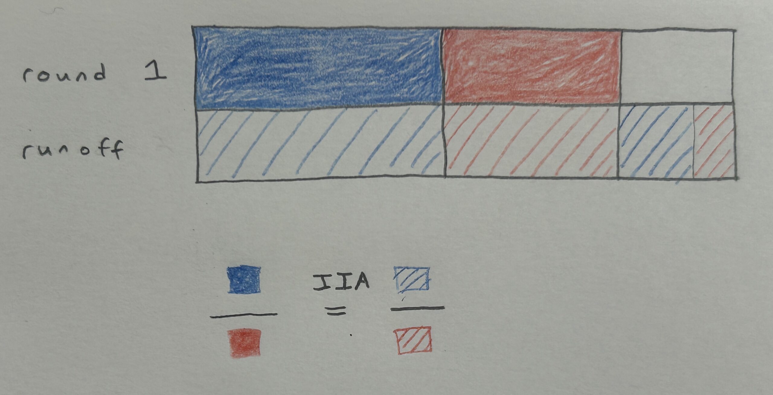
In fact, not only does logit model –> IIA (your homework to show), but IIA –> logit model. The latter direction is harder to show, see Luce (1959). For more, see Train (2009).

But then in reality, when you get the data nothing is formatted or works like in the textbooks, although they are helpful, most of time is spend like, extracting the information. And it’s much more complex. But the foundation is important and the references are good, I guess.
Fair point, Dre ! AI coding agents probably are quite useful with the reformatting data. But beyond that I agree that textbooks often make simplifying assumptions that are difficult to extend to real life situations.
I hadn’t read Train (2009) book before, but wow, looks really good at first glance. The chapter (8) on methods for maximum likelihood estimation is one of the most accessible and most comprehensive explanations of the topic I’ve come across. Nice!
I agree, Alex L ! The Train (2009) book is great. And Kenneth Train was also very kind and helpful in replying to my email questions.
To third the recommendation, back in grad school, we were heavily recommended (and I think used parts) of Train’s book.
Awesome, Paul ! I should write to Kenneth Train to share there are many fans here.
Thanks for the links, particularly to the RPDR example, which I will certainly share with the students in my Bayes class next semester!
To your point on IIA, it seems to me that one could introduce a “contrast matrix” K. Each cell in the matrix would model the degree to which that pair of options was “incompatible” or “attractive”. For example, entry K[i, j] would be the degree to which option i was incompatible with option j. You could then use this contrast matrix to weight the terms in the logit link function, to account for non-independence of alternatives. For example, if K[i, j] were positive, the presence of option i would exaggerate the value of option j (and vice versa) but would reverse it if K[i, j] were negative.
I believe such an approach is taken by Decision Field Theory to model non-independence, but I’m not aware of that approach being applied more generally. Also, it would only account for pairwise influences, not configural effects (eg, maybe option i only influences the attractiveness of option j in the presence of option k). Anyway, fun food for thought, thanks again!
Thanks, gec ! I hope your students enjoy the RPDR example. :)
I like your idea to depart from IIA. In Train (2009) chapter 4 they cover generalizing beyond IIA by allowing the utilities of different alternatives to be correlated. For example, two car alternatives (alone or carpool) might be correlated or two transit alternatives (train or bus) might be correlated. I can’t tell exactly how this compares to your idea, we would need to write out the exact models side by side. What do you think ?
Thanks for the pointer to the Train text!
I admit I hadn’t thought too deeply about my proposed approach, but I agree it sounds similar to allowing correlated utilities between components. To be more mathy about it, I think my original idea amounted to the following:
v_i = u_i + K[i,] %*% A
where v_i is the (pre-logit) value of option i, u_i is the “baseline” utility for option i, K[i,] is the i’th row of a matrix of contrast weights, and A is an indicator vector with 1’s the entries corresponding to the available choice alternatives and zeros elsewhere. The result is that v_i is an “adjusted” version of u_i that depends on the other available options.
Reading through Train, though, it sounds like a general correlated utilities model would require some numerical approximation, as described in the heteroskedastic logit section. Actually, reading that section, I realize now that I accidentally wrote a heteroskedastic logit model to address some category judgment data last year, I just didn’t recognize it as such at the time. That said, I ended up pursuing a different model in the end because of the onerous numerical approximations involved!
So that would argue in favor of approaches like the one you describe in your post today, which can capture some notion of correlated components while remaining tractable. I wonder if the silly contrast-weight approach I outline above would be able to strike a similar balance?
Thanks again!
Thanks, gec !
I think your approach is similar to Train (2009) Chapter 3 “Tests of IIA” ? (But your intent is not to test for IIA but to account for non-IIA.)