Paul Campos reminds us that just two years ago the Detroit Pistons were in the middle of a historic 28-game losing streak on the way to a 14-68 record (following up previous records of 17-65, 23-59, 20-50, and 20-46, so it’s not like that was much of an aberration), but now they’re leading the Eastern Conference with a 24-6 record, even though “The core talent group on that historically bad team still makes up the core talent of the present Detroit team, exactly two years later: Cade Cunningham, Jalen Duren, Ausar Thompson, Jaden Ivy, and Isaiah Stewart.”

Campos continues:

How did this happen? The answer is that all these players were extremely young two years ago: Cunningham and Stewart were 22, Ivy and Thompson were 21, and Duren was 20. Each of them has taken a huge leap forward in the subsequent two years . . .

I don’t know enough about basketball, and I haven’t been following the NBA at all lately, so I can’t comment on Campos’s judgment of the Pistons situation.

But in his post he also links to this old post of mine that I’d completely forgotten!, where I did a bunch of analysis to estimate how much information we get from 30 games in a season, compared to the information available from preseason betting odds.

I enjoy these posts where we go into the data and crunch through the R, and I know many of you like them too, so I thought I’d repeat it for you today for your holiday reading.

So here goes, from Christmas 2023:

Paul Campos points us to this discussion of the record of the Detroit professional basketball team:

The Detroit Pistons broke the NBA record for most consecutive losses in a season last night, with their 27th loss in a row. . . . A team’s record is, roughly speaking, a function of two factors:

(1) The team’s quality. By “quality” I mean everything about the team”s performance that isn’t an outcome of random factors, aka luck — the ability of the players, individually and collectively, the quality of the coaching, and the quality of the team’s management, for example.

(2) Random factors, aka luck.

The above-linked post continues:

How do we disentangle the relative importance of these two factors when evaluating a team’s performance to some point in the season? . . . The best predictor ex ante of team performance is the evaluation of people who gamble on that performance. I realize that occasionally gambling odds include significant inefficiencies, in the form of the betting public making sentimental rather than coldly rational wagers, but this is very much the exception rather than the rule. . . . the even money over/under for Detroit’s eventual winning percentage this season was, before the first game was played, a winning percentage of .340. To this point, a little more than third of the way through the season, Detroit’s winning percentage has been .0666. . . .

To the extent that the team has had unusually bad luck, then one would expect the team’s final record to be better. But how much better? Here we can again turn to the savants of Las Vegas et. al., who currently set the even money odds of the team’s final record on the basis of the assumption that it will have a .170 winning percentage in its remaining games.

Part of the confusion here is that we’re dealing with inference for p (the team’s “quality,” as summarized by the probability that they’d win against a randomly-chosen opponent on a random day) and also with predictions of outcomes. For the posterior mean, there’s no difference: under the basic model, the posterior expected proportion of future games won is equal to the posterior mean of p. It gets trickier when we talk about uncertainty in p.

How, then, could we take the beginning-of-season and current betting lines–which we will, for the purposes of our discussion here, identify as the prior and posterior means of p, ignoring systematic biases of bettor–and extract implied prior and posterior distributions? There’s surely enough information here to do this, if we use information from all 30 teams and calibrate properly.

Exploratory analysis

I started by going to the internet, finding various sources on betting odds, team records, and score differentials, and entering the data into this file. The latest Vegas odds I could find on season records were from 19 Dec; everything else came from 27 Dec.

Next step was to make some graphs. First, I looked at point differential and team records so far:

nba <- read.table("nba2023.txt", header=TRUE, skip=1)
nba$ppg <- nba$avg_points
nba$ppg_a <- nba$avg_points_opponent
nba$ppg_diff <- nba$ppg - nba$ppg_a
nba$record <- nba$win_fraction
nba$start_odds <- nba$over_under_beginning/82
nba$dec_odds <- nba$over_under_as_of_dec/82
nba$sched <- - (nba$schedule_strength - mean(nba$schedule_strength)) # signed so that positive value implies a more difficult schedule so far in season
nba$future_odds <- (82*nba$dec_odds - 30*nba$record)/52

pdf("nba2023_1.pdf", height=3.5, width=10)
par(mfrow=c(1,2), oma=c(0,0,2,0))
par(mar=c(3,3,1,1), mgp=c(1.5,.5,0), tck=-.01)
#
par(pty="s")
rng <- range(nba$ppg_a, nba$ppg)
plot(rng, rng, xlab="Points per game allowed", ylab="Points per game scored", bty="l", type="n")
abline(0, 1, lwd=.5, col="gray")
text(nba$ppg_a, nba$ppg, nba$team, col="blue")
#
par(pty="m")
plot(nba$ppg_diff, nba$record, xlab="Point differential", ylab="Won/lost record so far", bty="l", type="n")
text(nba$ppg_diff, nba$record, nba$team, col="blue")
#
mtext("Points per game and won-lost record as of 27 Dec", line=.5, side=3, outer=TRUE)
dev.off()

Here's a question you should always ask yourself: What do you expect to see?

Before performing any statistical analysis it's good practice to anticipate the results. So what do you think these graphs will look like?
- Ppg scored vs. ppg allowed. What do you expect to see? Before making the graph, I could have imagined it going either way: you might expect a negative correlation, with some teams doing the run-and-gun and others the physical game, or you might expect a positive correlation, because some teams are just much better than others. My impression is that team styles don't vary as much as they used to, so I was guessing a positive correlation.
- Won/lost record vs. point differential. What do you expect to see? Before making the graph, I was expecting a high correlation. Indeed, if I could only use one of these two metrics to estimate a team's ability, I'd be inclined to use point differential.

Aaaand, here's what we found:

Hey, my intuition worked on these! It would be interesting to see data from other years to see if I just got lucky with that first one.

Which is a better predictor of won-loss record: ppg scored or ppg allowed?

OK, this is a slight distraction from Campos's question, but now I'm wondering, which is a better predictor of won-loss record: ppg scored or ppg allowed? From basic principles I'm guessing they're about equally good.

Let's do a couple of graphs:

pdf("nba2023_2.pdf", height=3.5, width=10)
par(mfrow=c(1,3), oma=c(0,0,2,0))
par(mar=c(3,3,1,1), mgp=c(1.5,.5,0), tck=-.01)
#
par(pty="m")
rng <- range(nba$ppg_a, nba$ppg)
plot(rng, range(nba$record), xlab="Points per game scored", ylab="Won/lost record so far", bty="l", type="n")
abline(0, 1, lwd=.5, col="gray")
text(nba$ppg, nba$record, nba$team, col="blue")
#
par(pty="m")
plot(rng, range(nba$record), xlab="Points per game allowed", ylab="Won/lost record so far", bty="l", type="n")
abline(0, 1, lwd=.5, col="gray")
text(nba$ppg_a, nba$record, nba$team, col="blue")
#
par(pty="m")
plot(range(nba$ppg_diff), range(nba$record), xlab="Avg score differential", ylab="Won/lost record so far", bty="l", type="n")
abline(0, 1, lwd=.5, col="gray")
text(nba$ppg_diff, nba$record, nba$team, col="blue")
#
mtext("Predicting won-loss record from ppg, ppg allowed, and differential", line=.5, side=3, outer=TRUE)
dev.off()

Which yields:

So, about what we expected. To round it out, let's try some regressions:

library("rstanarm")
print(stan_glm(record ~ ppg, data=nba, refresh=0), digits=3)
print(stan_glm(record ~ ppg_a, data=nba, refresh=0), digits=3)
print(stan_glm(record ~ ppg + ppg_a, data=nba, refresh=0), digits=3)

The results:

            Median MAD_SD
(Intercept) -1.848  0.727
ppg          0.020  0.006

Auxiliary parameter(s):
      Median MAD_SD
sigma 0.162  0.021 
------
            Median MAD_SD
(Intercept)  3.192  0.597
ppg_a       -0.023  0.005

Auxiliary parameter(s):
      Median MAD_SD
sigma 0.146  0.019 
------
            Median MAD_SD
(Intercept)  0.691  0.335
ppg          0.029  0.002
ppg_a       -0.030  0.002

Auxiliary parameter(s):
      Median MAD_SD
sigma 0.061  0.008

So, yeah, points scored and points allowed are about equal as predictors of won-loss record. Given that, it makes sense to recode as ppg differential and total points:

print(stan_glm(record ~ ppg_diff + I(ppg + ppg_a), data=nba, refresh=0), digits=3)

Here's what we get:

               Median MAD_SD
(Intercept)     0.695  0.346
ppg_diff        0.029  0.002
I(ppg + ppg_a) -0.001  0.001

Auxiliary parameter(s):
      Median MAD_SD
sigma 0.062  0.009

Check. Once we include ppg_diff as a predictor, the average total points doesn't do much of anything. Again, it would be good to check with data from other seasons, as 30 games per team does not supply much of a sample.

Now on to the betting lines

Let's now include the Vegas over-unders in our analysis. First, some graphs:

pdf("nba2023_3.pdf", height=3.5, width=10)
par(mfrow=c(1,3), oma=c(0,0,2,0))
par(mar=c(3,3,1,1), mgp=c(1.5,.5,0), tck=-.01)
#
par(pty="s")
rng <- range(nba$start_odds, nba$record)
plot(rng, rng, xlab="Betting line at start", ylab="Won/lost record so far", bty="l", type="n")
abline(0, 1, lwd=.5, col="gray")
text(nba$start_odds, nba$record, nba$team, col="blue")
#
par(pty="s")
rng <- range(nba$record, nba$dec_odds)
plot(rng, rng, xlab="Won/lost record so far", ylab="Betting line in Dec", bty="l", type="n")
abline(0, 1, lwd=.5, col="gray")
text(nba$record, nba$dec_odds, nba$team, col="blue")
#
par(pty="s")
rng <- range(nba$start_odds, nba$dec_odds)
plot(rng, rng, xlab="Betting line at start", ylab="Betting line in Dec", bty="l", type="n")
abline(0, 1, lwd=.5, col="gray")
text(nba$start_odds, nba$dec_odds, nba$team, col="blue")
#
mtext("Won-lost record and over-under at start and in Dec", line=.5, side=3, outer=TRUE)
dev.off()

Which yields:

Oops--I forgot to make some predictions before looking. In any case, the first graph is kinda surprising. You'd expect to see an approximate pattern of E(y|x) = x, and we do see that--but not at the low end. The teams that were predicted to do the worst this year are doing even worse than expected. It would be interesting to see the corresponding graph for earlier years. My guess is that this year is special, not only in the worst teams doing so bad, but in them underperforming their low expectations.

The second graph is as one might anticipate: Betters are predicting some regression toward the mean. Not much, though! And the third graph doesn't tell us much beyond the first graph.

Upon reflection, I'm finding the second graph difficult to interpret. The trouble is that "Betting line in Dec" is the forecast win percentage for the year, but 30/82 of that is the existing win percentage. (OK, not every team has played exactly 30 games, but close enough.) What I want to do is just look at the forecast for their win percentage for the rest of the season:

pdf("nba2023_4.pdf", height=3.5, width=10)
par(mfrow=c(1,3), oma=c(0,0,2,0))
par(mar=c(3,3,1,1), mgp=c(1.5,.5,0), tck=-.01)
#
par(pty="s")
rng <- range(nba$record, nba$dec_odds)
plot(rng, rng, xlab="Won/lost record so far", ylab="Betting line of record for rest of season", bty="l", type="n")
abline(0, 1, lwd=.5, col="gray")
fit <- coef(stan_glm(future_odds ~ record, data=nba, refresh=0))
print(fit)
abline(fit, lwd=.5, col="blue")
text(nba$record, nba$future_odds, nba$team, col="blue")
#
dev.off()

Here's the graph:

The fitted regression line has a slope of 0.66:

            Median MAD_SD
(Intercept) 0.17   0.03  
record      0.66   0.05  

Auxiliary parameter(s):
      Median MAD_SD
sigma 0.05   0.01 

Next step is to predict the Vegas prediction for the rest of the season given the initial prediction and the team's record so far:

print(stan_glm(future_odds ~ start_odds + record, data=nba, refresh=0), digits=2)

            Median MAD_SD
(Intercept) -0.02   0.03 
start_odds   0.66   0.10 
record       0.37   0.06 

Auxiliary parameter(s):
      Median MAD_SD
sigma 0.03   0.00  

It's funny--everywhere we look, we see this 0.66. And 30 games is 37% of the season!

Now let's add into the regression the points-per-game differential, as this should include additional information beyond what was in the won-loss so far:

print(stan_glm(future_odds ~ start_odds + record + ppg_diff, data=nba, refresh=0), digits=2)

            Median MAD_SD
(Intercept) 0.06   0.06  
start_odds  0.67   0.09  
record      0.20   0.11  
ppg_diff    0.01   0.00  

Auxiliary parameter(s):
      Median MAD_SD
sigma 0.03   0.00 

Hard to interpret this one, as ppg_diff is on a different scale from the rest. Let's quickly standardize it to be on the same scale as the won-lost record so far:

nba$ppg_diff_std <- nba$ppg_diff * sd(nba$ppg_record) / sd(nba$ppg_diff)
print(stan_glm(future_odds ~ start_odds + record + ppg_diff_std, data=nba, refresh=0), digits=2)

             Median MAD_SD
(Intercept)  0.06   0.06  
start_odds   0.67   0.09  
record       0.20   0.11  
ppg_diff_std 0.17   0.10  

Auxiliary parameter(s):
      Median MAD_SD
sigma 0.03   0.00  

OK, not enough data to cleanly disentangle won-lost record and point differential as predictors here. My intuition would be that, once you have point differential, the won-lost record tells you very little about what will happen in the future, and the above fitted model is consistent with that intuition, but it's also consistent with the two predictors being equally important, indeed it's consistent with point differential being irrelevant conditional on won-lost record.

What we'd want to do here--and I know I'm repeating myself--is to repeat the analysis using data from previous years.

Interpreting the implied Vegas prediction for the rest of the season as an approximate weighted average of the preseason prediction and the current won-lost record

In any case, the weighting seems clear: approx two-thirds from starting odds and one-third from the record so far, which at least on a naive level seems reasonable, given that the season is about one-third over.

Just for laffs, we can also throw in difficulty of schedule, as that could alter our interpretation of the teams' records so far.

nba$sched_std <- nba$sched * sd(nba$record) / sd(nba$sched)
print(stan_glm(future_odds ~ start_odds + record + ppg_diff_std + sched_std, data=nba, refresh=0), digits=2)

             Median MAD_SD
(Intercept)  0.06   0.06  
start_odds   0.68   0.09  
record       0.21   0.11  
ppg_diff_std 0.17   0.10  
sched_std    0.04   0.03 

So, strength of schedule does not supply much information. This makes sense, given that 30 games is enough for the teams' schedules to mostly average out.

The residuals

Now that I've fit the regression, I'm curious about the residuals. Let's look:

fit_5 <- stan_glm(future_odds ~ start_odds + record + ppg_diff_std + sched_std, data=nba, refresh=0)
fitted_5 <- fitted(fit_5)
resid_5 <- resid(fit_5)
#
pdf("nba2023_5.pdf", height=5, width=8)
par(mar=c(3,3,1,1), mgp=c(1.5,.5,0), tck=-.01)
#
par(pty="m")
plot(fitted_5, resid_5, xlab="Vegas prediction of rest-of-season record", ylab="Residual from fitted model", bty="l", type="n")
abline(0, 0, lwd=.5, col="gray")
text(fitted_5, resid_5, nba$team, col="blue")
#
dev.off()

And here's the graph:

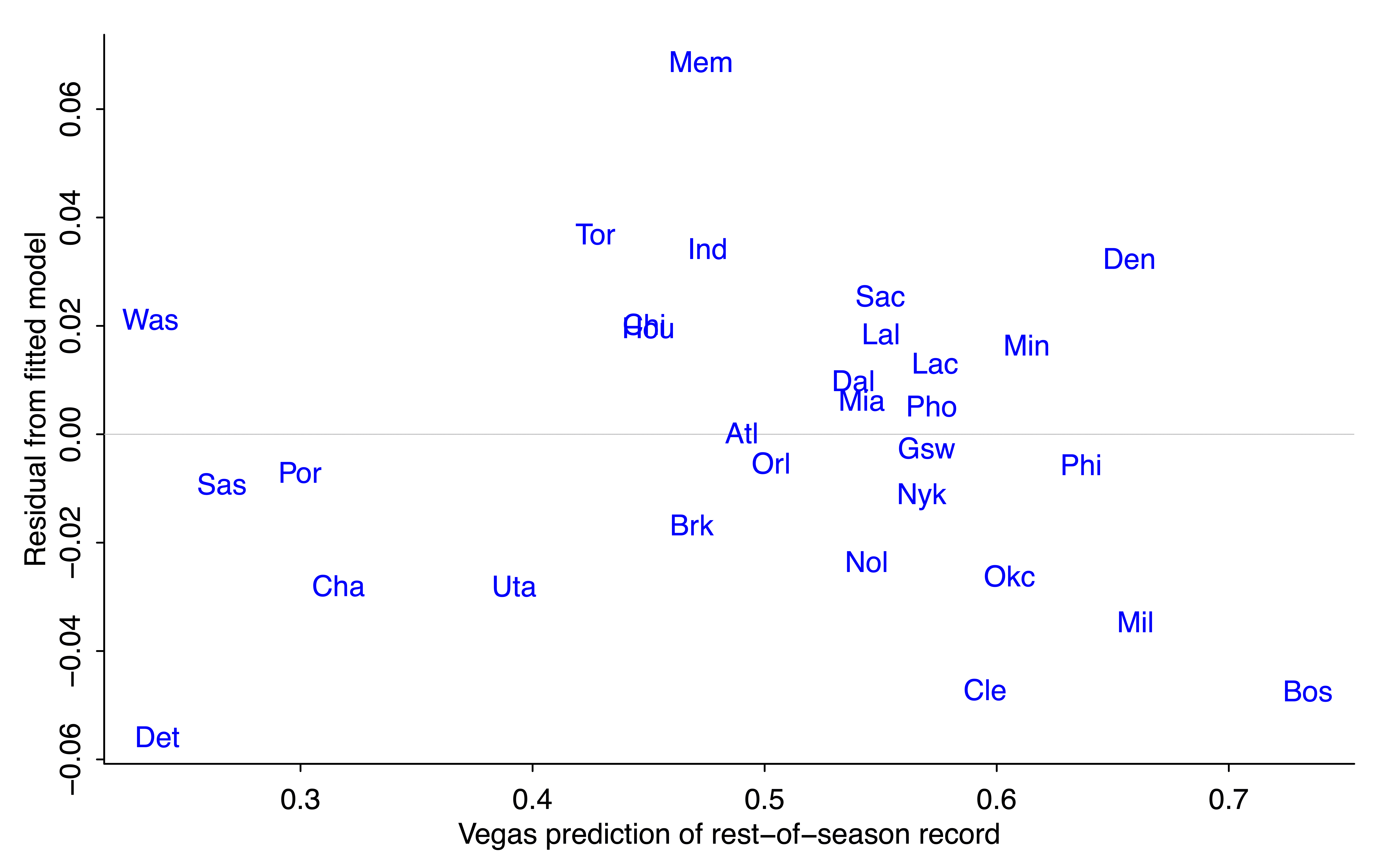
The residual for Detroit is negative (-0.05*52 = -2.6, so the Pistons are expected to win about 3 games less than their regression prediction based on prior odds and outcome of first 30 games). Cleveland and Boston are also expected to do a bit worse than the model would predict. On the other direction, Vegas is predicting that Memphis will win about 4 games more than predicted from the regression model.

I have no idea whassup with Memphis. The quick generic answer is that the regression model is crude, and bettors have other information not included in the regression.

Reverse engineering an implicit Bayesian prior

OK, now for the Bayesian analysis. As noted above, we aren't given a prior for team j's average win probability, p_j; we're just given a prior point estimate of each p_j.

But we can use the empirical prior-to-posterior transformation, along with the known likelihood function, under the simplifying assumption the 30 win-loss outcomes for each team j are independent with constant probability p_j for team j. This assumption that is obviously wrong, given that teams are playing each other, but let's just go with it here, recognizing that with full data it would be straightforward to extend to an item-response model with an ability parameter for each team (as here).

To continue, the above regression models show that the Vegas "posterior Bayesian" prediction of p_j after 30 games is approximately a weighted average of 0.65*(prior prediction) + 0.35*(data won-loss record). From basic Bayesian algebra (see, for example, chapter 2 of BDA), this tells us that the prior has about 65/35 as much information as data from 30 games. So, informationally, the prior is equivalent to the information from (65/35)*30 = 56 games, about two-thirds of a season worth of information.

Hey--what happened??

But, wait! That approximate 2/3 weighting for the prior and 1/3 weighting of the data from 30 games is the opposite of what Campos reported, which was a 1/3 weighting of the prior and 2/3 of the data. Recall: prior estimated win probability of 0.340, data win rate of 0.067, take (1/3)*0.340 + (2/3)*0.067 and you get 0.158, which isn't far from the implied posterior estimate of 0.170.

What happened here is that the Pistons are an unusual case, partly because the Vegas over-under for their season win record is a few percentage points lower than the linear model predicted, and partly because when the probability is low, a small percentage-point change in the probability corresponds to a big change in the implicit weights.

Again, it would be good to check all this with data from other years.

Skill and luck

There's one more loose end, and that's Campos taking the weights assigned to data and prior and characterizing them as "skill" and "luck" in prediction errors. I didn't follow that part of the reasoning at all so I'll just let it go for now. Part of the problem here is in one place Campos seems to be talking about skill and luck as contributors to the team's record, and in another place he seems to considering them as contributors to the difference between preseason predictions and actual outcomes.

One way to think about skill and luck in a way that makes sense to me is within an item-response-style model in which the game outcome is a stochastic function of team abilities and predictable factors. For example, in the model,

score differential = ability of home team - ability of away team + home-field advantage + error,

the team abilities are in the "skill" category and the error is in the "luck" category, and, ummm, I guess home-field advantage counts as "skill" too? OK, it's not so clear that the error in the model should all be called "luck." If a team plays better against a specific opponent by devising a specific offensive/defensive plan, that's skill, but it would pop up in the error term above.

In any case, once we've defined what is skill and what is luck, we can partition the variance of the total to assign percentages to each.

Another way of looking at this is to consider the extreme case of pure luck. If outcomes determined only by luck, then each game is a coin flip, and we'd see this in the data because the team win proportions after 30 games would follow a binomial distribution with n=30 and p=0.5. The actual team win proportions have mean 0.5 (of course) and sd 0.18, as compared to the theoretical mean of 0.5 and sd of 0.5/sqrt(30) = 0.09. That simple calculation suggests that skill is (0.18/0.09)^2 = 4 times as important as luck when determining the outcome of 30 games.

And maybe I'm getting just getting this all tangled myself. The first shot at any statistical analysis often will have some mix of errors in data, modeling, computing, and general understanding, with that last bit corresponding to the challenge of mapping from substantive concepts to mathematical and statistical models. Some mixture of skill and luck, I guess.

Summary

1. Data are king. In the immortal words of Hal Stern, the most important aspect of a statistical analysis is not what you do with the data, it’s what data you use. I could do more than Campos did, not so much because of my knowledge of Bayesian statistics but because I was using data from all 30 teams.

2. To continue with that point, you can do lots better than me by including data from other years.

3. Transparency is good. All my data and code are above. I might well have made some mistakes in my analyses, and, in any case, many loose ends remain.

4. Basketball isn't so important (hot hand aside). The idea of backing out an effective prior by looking at information updating, that's a more general idea worth studying further. This little example is a good entry point into the potential challenge of such studies.

5. Models can be useful, not just for prediction but also for understanding, as we saw for the problem of partitioning outcomes into skill and luck.