It’s time for football (aka soccer) World Cup Qatar 2022 and statistical predictions!
This year me and my collaborator Vasilis Palaskas implemented a diagonal-inflated bivariate Poisson model for the scores through our `footBayes` R CRAN package (depending on the `rstan` package), by considering as a training set more than 3000 international matches played during the years’ range 2018-2022. The model incorporates some dynamic-autoregressive team-parameters priors for attack and defense abilities and the Coca-Cola/FIFA rankings differences as the only predictor. The model, firstly proposed by Karlis & Ntzoufras in 2003, extends the usual bivariate Poisson model by allowing to inflate the number of draw occurrences. Weakly informative prior distributions for the remaining parameters are assumed, whereas sum-to-zero constraints for attack/defense abilities are considered to achieve model identifiability. Previous World Cup and Euro Cup models posted in this blog can be found here, here and here.
Here is the new model for the joint couple of scores (X,Y,) of a soccer match. In brief:

We fitted the model by using HMC sampling, with 4 Markov Chains, 2000 HMC iterations each, checking for their convergence and effective sample sizes. Here there are the posterior predictive matches probabilities for the held-out matches of the Qatar 2022 group stage, played from November 20th to November 24th, along with some ppd ‘chessboard plots’ for the exact outcomes in gray-scale color (‘mlo’ in the table denotes the ‘most likely result’ , whereas darker regions in the plots correspond to more likely results):
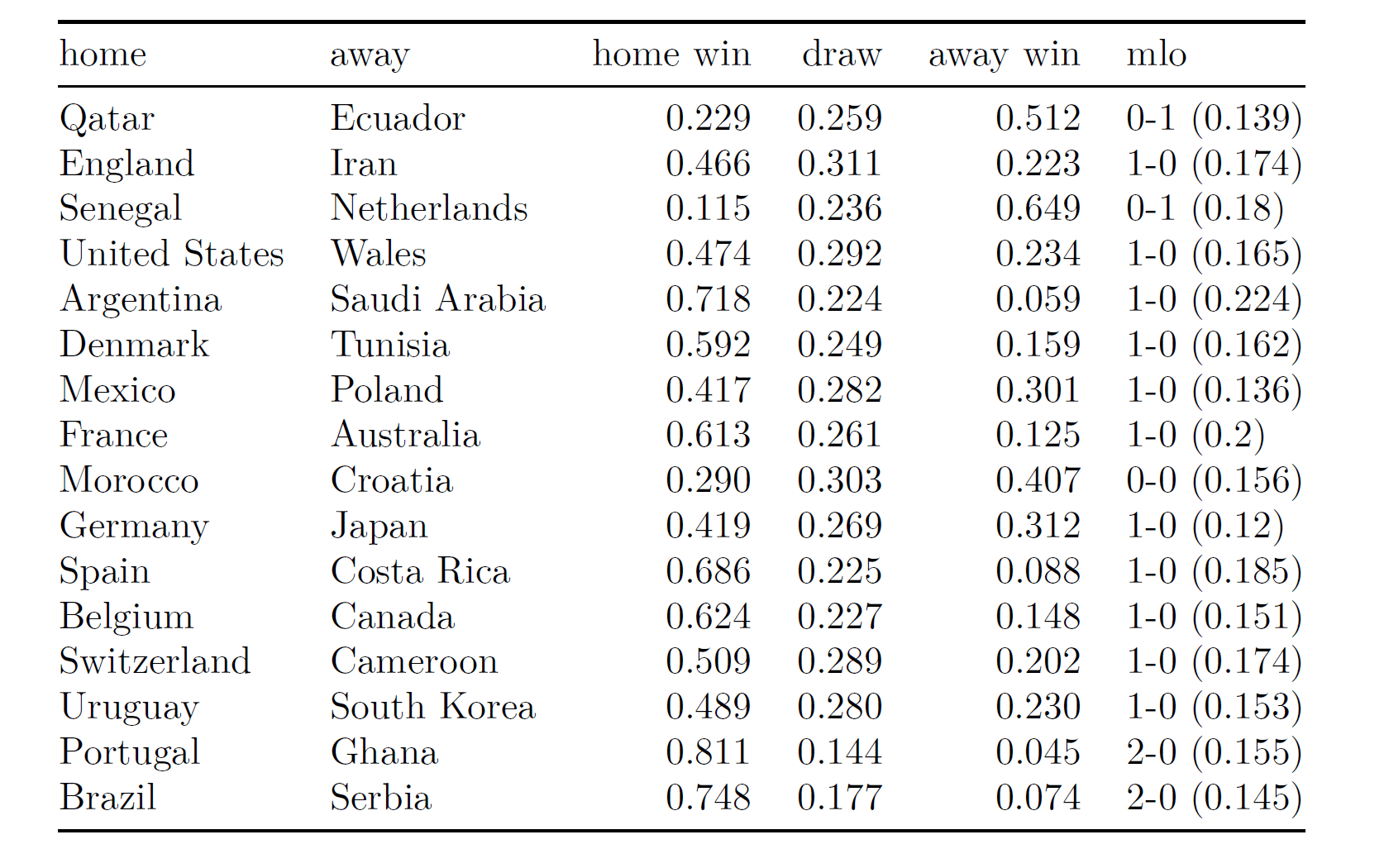

Better teams are acknowledged to have higher chances in these first group stage matches:
- In Portugal-Ghana, Portugal has an estimated winning probability about 81%, whereas in Argentina-Saudi Arabia Argentina has an estimated winning probability about 72%. The match between England and Iran seems instead more balanced, and a similar trend is observed for Germany-Japan. USA is estimated to be ahead in the match against Wales, with a winning probability about 47%.
Some technical notes and model limitations:
- Keep in mind that ‘home’ and ‘away’ do not mean anything in particular here – the only home team is Qatar! – but they just refer to the first and the second team of the single matches. ‘mlo’ denotes the most likely exact outcome.
- The posterior predictive probabilities appear to be approximated at the third decimal digit, which could sound a bit ‘bogus’… However, we transparently reported the ppd probabilities as those returned from our package computations.
- One could use these probabilities for betting purposes, for instance by betting on that particular result – among home win, draw, or away win – for which the model probability exceeds the bookmaker-induced probability. However, we are not responsible for your money loss!
- Why a diagonal-inflated bivariate Poisson model, and not other models? We developed some sensitivity checks in terms of leave-one-out CV on the training set to choose the best model. Furthermore, we also checked our model in terms of calibration measures and posterior predictive checks.
- The model incorporates the (rescaled) FIFA ranking as the only predictor. Thus, we do not have many relevant covariates here.
- We did not distinguish between friendly matches, world cup qualifiers, euro cup qualifiers, etc. in the training data, rather we consider all the data as coming from the same ‘population’ of matches. This data assumption could be poor in terms of predictive performances.
- We do not incorporate any individual players’-based information in the model, and this also could represent a major limitation.
- We’ll compute some predictions’ scores – Brier score, pseudo R-squared – to check the predictive power of the model.
- We’ll fit this model after each stage, by adding the previous matches in the training set and predicting the next matches.
This model is just an approximation for a very complex football tornament. Anyway, we strongly support scientific replication, and for such reason the reports, data, R and RMarkdown codes can be fully found here, in my personal web page. Feel free to play with the data and fit your own model!
And stay tuned for the next predictions in the blog. We’ll add some plots, tables and further considerations. Hopefully, we’ll improve predictive performance as the tournament proceeds.
Leo:
Whassup with those graphs on the bottom? Is there a chance that the U.S. scores 2.5 goals? I suggest you put all those on a common scale, also make them square. I’d say show 0, 1, 2, 3, 4+, so you don’t have to worry about plotting the unlikely events of teams scoring 6 goals. Also please please please please please don’t list these alphabetically! I recommend more logical order such as close games first and blowouts later, or vice versa. Even better would be a 2-way grid with countries listed from best to worst. If you use small multiples (i.e., exact same graph format for each matchup), you can actually make those match-probability plots very small and have only a small amount of space between them: you’d be surprised at how many you can fit on a single plot. Also I recommend plotting as favorite vs. underdog, not home vs. away, given that the games are being played in essentially neutral turf for most of the teams. I could say more, but that’s enough for now.
Andrew:
very good points, thanks! We’re gonna work a bit on the plot codes of our package over the next days. The 2-way grid with countries listed from best to worst, along with plotting as favorite vs underdog in place of ‘home’ and ‘away’, could actually be the best solution. Let’s try to take the most from the ‘ggplot2’ functionalities in order to improve the package.
We’ll adopt similar changes to the table as well. However, here matches are displayed in terms of their chronological order, which could maybe seem a reasonable and decent order (at least for soccer fans…). We could anyway include an optional argument in the function to establish the order of visualization of the matches.
I had to guess which country was the “x” axis and which the “y”, which should not be necessary for a graph. I agree with Andrew that the graphs should be square. I like the gray-scale probability and the overall look, though!
This means you overfit, it would be interesting to get an update comparing the final predictive skill vs what you saw on the cv holdouts.
Anoneuoid:
Thanks, the comparison you suggest is interesting. However, I do not think this model overfits much the training data. We just selected the best model according to the LOO criterion and some pp checks. To be transparent, there were not large differences between the diagonal-inflated and the ‘regular’ bivariate Poisson model.
When I first learned ML I was really surprised how much overfitting I could achieve via the black magic of tuning hyperparameters repeatedly on the same data to improve CV fit. Selecting a model is essentially one way to do that.
Also I didn’t look at your code but most of the time people don’t make sure the validation data came after the training data. Thus they have future data predicting the past.
The best solution seems to be splitting the data into training, validation, and a final holdout by datetime. Then report the skill on that final holdout after it was checked only once.
This simulates predicting the future as close as I have seen, but of course the tempation is almost irresistable to then mess with the model if you see poorer results.
Running many models and choosing the best indeed biases the cross validated error downwards relative to true out of sample performance. But holding more data out in development also biases the cross validated error estimator upwards because you’re evaluating models trained on less data than you actually have, and having a single holdout also increases variance of the cross validation estimator relative to procedures like leave p-out or k-fold. On yet a third hand, procedures like LOO may also bias cross validated error upwards because the holdout element is always underrepresented relative to the true distribution, though this bias disappears asymptotically.
In addition, the goal of estimating out of sample predictive skill is different from the goal of model selection. Bias relative to true out of sample performance is not necessarily a problem at all for model selection as long as the bias is the same across candidate models—you only need it to give a correct order for the candidate models. In fact, more bias for out of sample error estimation may actually improve model selection by making differences easier to resolve. Anyways, in this context, the true holdout cannot help the model selection decision (since by construction, you’re not deciding anything with it) but it can hurt because:
1. the variance of the estimator is higher due to less data being used for validation during model selection
2. the holdout induced bias does not apply equally across methods; it has a bigger effect on more data hungry methods
To give an analogy, suppose I bring 10000 high school kids and have them shoot up to 100 times from the 3 point line in 2 minutes, then pick the one who gets the highest score. If I then have the winner of this selection method do the same competition again, they will most likely not perform as well as they did the first time because of regression to the mean; the best stage 1 performance is biased upwards. However, the winner is still the choice that maximizes expected stage 2 performance conditional on stage 1 performance; the winner is still the best choice based on the information available.
To take this analogy even further, suppose I’m getting too many candidates in the region of 98-100 baskets. A reasonable choice might be to have the candidates shoot from half court in stage 1. It produces a biased estimate of stage 2 performance because half court is harder, but is nonetheless more likely to select the best stage 2 shooter.
There is no general guidance or guarantee outside the land of asymptotia, which we can all agree is a myth. But it’s important to distinguish between the different goals of cross validation.
Side note:
Side note: this is quite a bit harder in the fully bayesian world than in ML point estimation since full bayes does not maximize a quantity closely related to your CV metric. It’s not built to maximize any quantity at all, though if you’re being pedantic you could say it maximizes the negative KL divergence between the parameters sampled and the theoretical posterior distribution.
But of course it’s still possible to overfit if you’re determined to.
Leo:
Also, you say your model gives predictions, so can you give predictions of the probability of each of the teams winning it all? That’s what we all want to know!
This is one of the big advantages I see of Bayesian methods over frequentist in applied problems where you want to do ‘something’ with your estimates – that propagating uncertainties through downstream calculations is easy using MCMC draws (in this case calculating posterior distributions for the winner of the world cup).
(Shameless plug, or useful example – you decide) I did similar here for track cycling at the Tokyo olympics, where I used Stan to estimate outcomes for individual races, and from this derived posterior probabilities for the gold medal winner – and ultimately a betting strategy to go with it.
https://www.infreq.com/posts/2021-08-03-tokyo-2020-iii/
Andrew:
eheh, yeah, I know, that would be the hottest prediction!
Our code does not support yet this ‘final winner’ prediction, although we could try to work on it asap. To do this, we’d need to simulate the Qatar 2022 tournament progress 10000 or 100000 times (or even more) in terms of model ppd and count the winning frequencies for each team to get some approximated winning probabilities.
Then, final winning probabilities should be updated after each stage.