Paul Kedrosky asks:
Have you written anything on approximate Bayesian computation? It is seemingly all the rage in ecology and population genetics, and this recent paper uses it heavily to come to some heretical conclusions.
I passed this over to Lizzie who wrote:
Fun paper! Unfortunately, I too do not know much about this myself but I have two examples where I have heard of using it, both of which I think have some similar issues of exponentially increasing number of possible branches taken (e.g., Coalescent theory of pop gen and Lévy flight models). I don’t know the math of these models well enough to know what exactly makes the likelihood so expensive to calculate and I don’t really see authors explaining that on quick glance. My very gut reaction is that these are inherently non-identifiable models ….
Lizzie also pointed to figure 1 in this paper which I’ve reproduced above. And she asked, “What makes something ‘approximate’ Bayesian? And is it different than being ‘approximately’ Bayesian?” I replied that, except in some very simple models, all inferences, Bayesian or otherwise, are approximate, and all computations are approximate too, in the sense that you can’t really get exact draws from the posterior distribution or closed forms for posterior expectations or intervals.
And Lizzie connected us to Geoff Legault, who wrote:
The paper is also a mystery to me, but I do think ABC methods, or more broadly, simulation-based inference can be useful if done carefully and with full awareness of its many limitations.
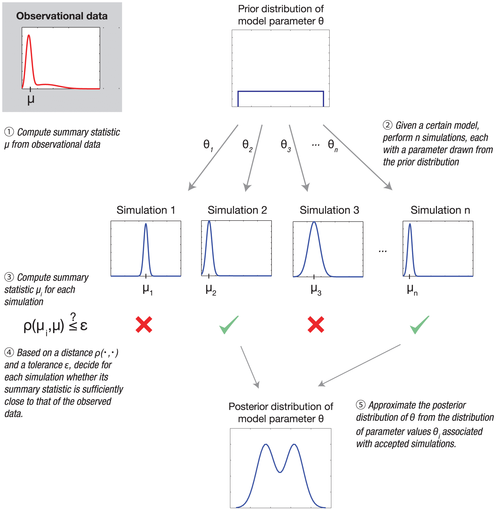
In ecology, there are many “models” that are easily simulated, that in principle have likelihood/probability functions, but those likelihoods are not available or they cannot possibly be computed. For example, certain kinds of stochastic, spatially-explicit population models would require working with transition matrices that are too large for any computer that currently exists or will ever exist (probably). I gather some models in physics also such intractable likelihoods. In those cases, the idea is to use the simulator to either approximate the likelihood or simply to learn more about your model. Most applications of simulation-based inference that I’ve seen opt for the latter: parameter values are sampled from a prior distribution, data is simulated with them, distances between several summary statistics of simulated and real data are computed, and those (parameter) samples with distances below some tolerance level are retained. To me, the reliance on distances between summary statistics feels much more “approximate” than the usual approximations we accept when making most inferences.
In addition to the paper Lizzie linked, I highly recommend this recent review of simulation-based inference.
And John Wakeley adds:
Here’s ABC in a nutshell from the perspective of population genetics. Ideally you want the likelihood of the full data, but this is too complicated to compute analytically. It is even too complicated to compute using simulations because the data have too many dimensions and you might not even be quite sure what to measure. An example would be the whole genomes of a sample of individuals. Also, you are interested in particular model(s) with particular parameters which might not be enough to determine all aspects of the data. These issues are of course in common to all sorts of inference problems. In ABC, there are two or three ways in which approximations are made. The first, also in common with many inference methods, is dimension reduction. You choose some quantities to calculate from the full data, ones which capture what you think are important axes of variation, relevant to your model(s) and parameters. The second is to choose a tolerance level, which you’ll use to estimate the probability of the reduced data by a rejection method. Specifically, for a given set of parameter values, you compute the fraction of simulation replicates which produce values of these quantities close enough to your observed ones to be acceptable. Obviously this requires some finesse: too loose a tolerance means tossing out much to the information you’ve got, and too tight a tolerance can put you back in situation you were trying to avoid in the first place (i.e. if almost no simulation replicates will give exactly the observed values of your quantities). A wrinkle in population genetics, due to genomes being more-or-less digital, is that most of the commonly used quantities are discrete rather than continuous, so tolerances should be chosen accordingly but that’s not necessarily a simple matter depending on the particular quantities. The third point of approximation is the choice of the number of simulation replicates. I suppose this could also bring up subtleties, e.g. the unevenness of errors in estimating the likelihoods for different sets of parameters values.
So there you have it. This discussion makes me think that there could be some useful ways to extend our Bayesian workflow to simulation-based models.
Ever since Rubin pointed out the conceptual clarity of Bayes thought of as two stage sampling – draw from the prior, then draw data and then condition of the data in hand (rejection sampling) it has been a pedagogical option for toy problems.
Recently it has become feasible to do many analyses that would be suitable for teaching a first course allowing MCMC to covered afterwards and conjugacy maybe skipped over all together.
Also the two stage sampling process is already part of the Bayesian Work flow https://betanalpha.github.io/assets/case_studies/principled_bayesian_workflow.html#12_Computational_Faithfulness
Keith:
Yes, this is the simulation-based calibration technique that was covered in the 2006 paper by Cook, Rubin, and myself (see also here). Cook was a Ph.D. student of Rubin and this paper derives from her Ph.D. thesis. So it’s been part of Bayesian workflow for awhile, at least in principle. In practice, we will often just simulate fake data from the model once or twice, which can be enough to show gross problems of computation. One challenge is that real computation is just about always approximate; a current area of research is to quantify the magnitude of departures from calibration rather than just setting calibration as a pure goal.
I remember referencing that 2006 paper as the first practical (as opposed to just conceptual) use of what became known as ABC.
Keith:
I don’t know that this 2006 paper was so practical in practice, but I agree that it’s practical in theory.
Can something be practical in theory? Seems like it can’t be practical unless it is…um….put into practice.
Anon:
Some ideas aren’t even practical in theory! By “practical in theory,” I mean that it has a close enough connection to practical goals to be potentially useful.
The population genetic motivation for ABC as in Tavaré et al. (1997) is not in recreating philogenies but in inferring the entire sequence of mutations along the branches of a given philogeny tree starting from the most recent common ancestor. A proper entry to the topic of ABC is the recent Handbook of Approximate Bayesian Computation (CRC Press), with most chapters available on arXiv.
Several years ago I participated in a phylogenetics seminar where the biologists were interested in using Bayesian methods. I haven’t participated in several years, but looking up some things more recent, I came across the following that show some of the types of things the biologists are interested in:
This is the website of someone who was a graduate student then: https://wright-lab.com/
Here’s one that sounds really ambitious: https://www.evoio.org/wiki/Phylotastic#What.27s_phylotastic
I think its a mistake to have used ABC as the catchy acronym. There’s nothing approximate about it any more than any other Bayesian method. Its just Bayesian inference on simulation models. I think we need to spend a lot more effort on this. Lots of useful models are nondifferentiable. For example agent based models of animal migration patterns or of species competition or pandemics or the latency induced by mismatched queuing behavior of packet delivery over IP networks. We know how to write iterative simulations of these things but they involve generating random numbers and making decisions based on the outcomes and these will never be the sort of thing you can do HMC on. We need fast convergence of inference chains for this kind of model.
But if you are conditioning on summaries that are not sufficient, then it is an approximation.
No its just a model for that particular summary. “All models are wrong” is another way of saying “all models are approximations” there’s nothing more approximate about this class of model, its just a different kind of approximation. Its like saying “accounting” is “approximate financial computation” because we don’t include the loose change under the couch cushions or have an accounts receivable for our friend who borrows $10 to buy lunch or because occasionally banks have to write down millions of dollars in fraudulent charges due to credit card fraud.
The issue comes about because to predict the summaries we first predict the details and then summarize. Its this sense in which people wrongfully think of the computation as approximate for something else. in most cases we are better off thinking of the simulation model as just a means to predict summaries. Like molecular dynamics isn’t supposed to predict where each molecule is in your jar of honey, its supposed to predict how the viscosity changes with temperature. Those are both summary quantities and are not “sufficient”, for example there is also bulk modulus, and coefficient of thermal expansion, and vapor pressure and molecular chain breakage rate, and calorie content and crystallized fraction and…
Yup, all models are wrong but some are useful. With conditioning on some (perhaps poor) choice of summaries rather than the data itself, one needs to worry if that has made it less useful. There can be a large loss of information e.g. skewness.
Somehow it seems like my reply was lost.
I believe that your concern exists equally with simulation based models and with more “analytical” models (such as algebraic equations or ODEs) and by calling ABC “approximate” and treating those others as if they were “exact” we give a very STRONGLY misleading slant on things which can lead people to not use simulation models where they would be appropriate, or to have too much confidence in their analytical models.
If we write an ODE for COVID infections and then fit it to case counts without consideration that case counts is a biased summary of the “real” data, then we get the same bias problems you mention and it has nothing to do with whether we used ABC methods. The same is true if we write an analytical model that includes information about undercounting infections, but instead of fitting it individually to every metropolitan area in the country we fit it to a summary of the entire country. Again, this has nothing to do with whether we are running a “simulation” or using an algebraic equation.
Agreed, but again this is no different from any other model. If we condition on confirmed COVID cases we underestimate infections, even if we use an analytical ODE model for the predictions of infections per day. Its nothing to do with “ABC” as a method its just a general problem in modeling, we need to choose the appropriate level of detail.
My concern is that by giving the misimpression that ABC is somehow “different” it discourages the use of simulation models and encourages a false sense of security about non simulation models. But there is ultimately no logical difference between writing a model in terms of a detailed simulation that you summarize explicitly and a non detailed equation that predicts the summary directly. They both have the same issues to consider.
> discourages the use of simulation models and encourages a false sense of security about non simulation models
We definitely don’t want that and simulation is just a different medium of math and all mediums have there advantages and disadvantages.
But choosing the wrong summary, even if it can be worked analytical is a loss of information.
This approach is nearly identical to a method known as “indirect inference” in econometrics. In those applications, the likelihood for the economic models may be too difficult to evaluate analytically. But there may be some simple “auxiliary” statistics are easily computable using only the data (e.g. regression coefficients, means, variances, etc.). The idea of indirect inference is to simulate data from the model, and search for parameter values that minimize the distance between the simulated auxiliary statistics and the observed auxiliary statistics. This procedure is consistent under some regularity conditions (one being that there are at least as many auxiliary statistics as parameters being estimated).
Cosma Shalizi has a nice blog post about it with references. He also mentions the similarity to approximate Bayesian computation: http://bactra.org/notebooks/indirect-inference.html