
tl;dr: Their 95% interval for the infection rate, given the data available, is [0.7%, 1.8%]. My Bayesian interval is [0.3%, 2.4%]. Most of what makes my interval wider is the possibility that the specificity and sensitivity of the tests can vary across labs. To get a narrower interval, you’d need additional assumptions regarding the specificity and sensitivity of the particular experiment done for that report.
1. Background
A Stanford research team gave coronavirus tests for a sample of people from Santa Clara County, California. 1.5% of the people in the sample tested positive, but there were concerns about false positives, as well as about possible sampling bias. A couple weeks later, the Stanford team produced a new report with additional information on false positive and false negative rates. They also produced some new confidence intervals, but their procedure is pretty complicated, as it has to simultaneously handle uncertainties in three different probabilities.
This seems like a good case for Bayesian analysis, so I decided to do it.
2. The Stan model and R script
First I created a file, santaclara.stan:
data {
  int y_sample;
  int n_sample;
  int y_spec;
  int n_spec;
  int y_sens;
  int n_sens;
}
parameters {
  real<lower = 0, upper = 1> p;
  real<lower = 0, upper = 1> spec;
  real<lower = 0, upper = 1> sens;
}
model {
  real p_sample;
  p_sample = p * sens + (1 - p) * (1 - spec);
  y_sample ~ binomial(n_sample, p_sample);
  y_spec ~ binomial(n_spec, spec);
  y_sens ~ binomial(n_sens, sens);
}
It’s easy to do this in Rstudio: just click on File, New File, and then there’s a Stan File option!
Then I ran this R script:
library("cmdstanr")
library("rstan")
stanfit <- function(fit) rstan::read_stan_csv(fit$output_files())

sc_model <- cmdstan_model("santaclara.stan")

# Using data from Bendavid et al. paper of 11 Apr 2020

fit_1 <- sc_model$sample(data = list(y_sample=50, n_sample=3330, y_spec=369+30, n_spec=371+30, y_sens=25+78, n_sens=37+85), refresh=0)

# Using data from Bendavid et al. paper of 27 Apr 2020

fit_2 <- sc_model$sample(data = list(y_sample=50, n_sample=3330, y_spec=3308, n_spec=3324, y_sens=130, n_sens=157), refresh=0)

print(stanfit(fit_1), digits=3)
print(stanfit(fit_2), digits=3)
The hardest part here was figuring out what numbers to use from the Bendavid et al. papers, as they present several different sources of data for sensitivity and specificity. I tried to find numbers that were as close as possible to what they were using in their reports.
3. Results
And here's what came out for the model fit to the data from the first report:
         mean se_mean    sd     2.5%      25%      50%      75%    97.5% n_eff  Rhat
p       0.010   0.000 0.005    0.001    0.007    0.011    0.014    0.019  1198 1.005
spec    0.993   0.000 0.003    0.986    0.991    0.994    0.996    0.999  1201 1.004
sens    0.836   0.001 0.035    0.758    0.814    0.838    0.861    0.897  1731 1.000
lp__ -338.297   0.054 1.449 -342.043 -338.895 -337.900 -337.258 -336.730   721 1.005
And for the model fit to the data from the second report:
         mean se_mean    sd     2.5%      25%      50%      75%    97.5% n_eff  Rhat
p       0.013   0.000 0.003    0.007    0.010    0.012    0.015    0.019  2598 1.000
spec    0.995   0.000 0.001    0.992    0.994    0.995    0.996    0.997  2563 1.001
sens    0.822   0.001 0.031    0.759    0.802    0.823    0.844    0.879  2887 1.000
lp__ -446.187   0.031 1.307 -449.546 -446.810 -445.841 -445.221 -444.718  1827 1.001
The parameter p is the infection rate in the population for which the data can be considered a random sample.
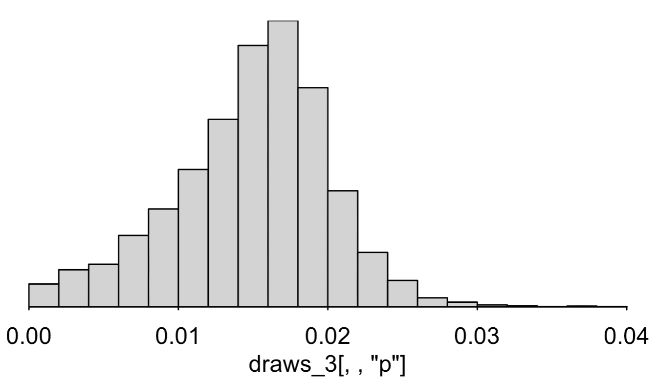
In the model fit to the data from the first report, the 95% interval for p is [0.001, 0.019]---that is, the data are consistent with an underlying infection rate of between 0 and 2%. The lower bound of the interval does not go all the way to zero, but that's just an artifact of summarizing inferences by a central interval. For example, we can plot the posterior simulation draws:
draws_1 <- fit_1$draws()
hist(draws_1[,,"p"])
And you get this:

In the model fit to the data from the second report, the 95% interval for p is [0.007, 0.019]---that is, the data are consistent with an underlying infection rate of between 0.7% and 2%.
4. Notes
a. As discussed in my earlier post, this is all based on the assumption that the sensitivity and specificity data represent independent tests with constant probability---that's implicit in the binomial model in the above Stan program. If you start allowing the specificity to vary from one experiment to another, then you can't just pool---you'd want to fit a hierarchical model---and that will end up giving you a wider uncertainty interval for p.
b. Also as discussed in my earlier post, I'm ignoring the weighting done by Bendavid et al. to adjust for differences between the sample and population. I just have too many questions about what they did, and their data are not available. I think the best way to do this adjustment would be using multilevel regression and poststratification. It would be easy to do this with a slight expansion of the above Stan program, so if someone has these data, they could do it. More to the point, this is the sort of adjustment that could and should be done in future studies with nonrepresentative samples.
c. I'm also ignoring the possibility, which we've also discussed, that people with symptoms or at higher risk of infection were more likely to respond to the survey.
d. The Stan model was super easy to write. It did take a few minutes to debug, though. In addition to some simple typos, I had an actual mistake. Originally, I had "p_sample = p*sens + (1-p)*(1-spec)" as "p_sample = p*sens + (1-p)*spec". That's not right at all! When I ran that model, it had terrible mixing and the inferences made no sense. I wasn't sure what was wrong, so to debug I did the following simplifications:
- First, I simply set p_sample = p;. This ran fine and it gave the correct inference for p (ignoring the corrections for sensitivity and specificity) and the right inferences for sens and spec as well.
- Then I got rid of the second term in the expression, so just p_sample = p*sens. This worked too. So the sensitivity adjustment did not seem to be causing the problem.
- I was then trying to figure out how to check the specificity correction, when I noticed that my formula was wrong so I fixed it.
The folk theorem wins again!
e. The statistical analysis is not magic. It's only as good as its assumptions, and points a, b, and c above suggest problems with the assumptions. The point of the analysis is to summarize the uncertainty given the data, if the assumptions were true. So in practice it should be an understatement of our actual uncertainty.
5. Hierarchical model
I was curious about the variation in sensitivity and specificity among the different datasets (13 specificity studies and 3 sensitivity studies) listed in the updated report. So I fit a hierarchical model allowing these two parameters to vary. I set up the model so that the specificities from the Santa Clara experiment and the 13 other studies were drawn from a common distribution, and the same for the sensitivities from the Santa Clara experiment and the 3 other studies.
Here's the Stan program, which I put in the file santaclara_hierarchical.stan:
data {
  int y_sample;
  int n_sample;
  int J_spec;
  int y_spec [J_spec];
  int n_spec [J_spec];
  int J_sens;
  int y_sens [J_sens];
  int n_sens [J_sens];
}
parameters {
  real<lower = 0, upper = 1> p;
  vector[J_spec] e_spec;
  vector[J_sens] e_sens;
  real mu_spec;
  real<lower = 0> sigma_spec;
  real mu_sens;
  real<lower = 0> sigma_sens;
}
transformed parameters {
  vector[J_spec] spec;
  vector[J_sens] sens;
  spec = inv_logit(mu_spec + sigma_spec * e_spec);
  sens = inv_logit(mu_sens + sigma_sens * e_sens);
}
model {
  real p_sample;
  p_sample = p * sens[1] + (1 - p) * (1 - spec[1]);
  y_sample ~ binomial(n_sample, p_sample);
  y_spec ~ binomial(n_spec, spec);
  y_sens ~ binomial(n_sens, sens);
  e_spec ~ normal(0, 1);
  e_sens ~ normal(0, 1);
  sigma_spec ~ normal(0, 1);
  sigma_sens ~ normal(0, 1);
}
This model has weakly-informative half-normal priors on the between-experiment standard deviations of the specificity and sensitivity parameters.
In R, I compiled, fit, and printed the results:
sc_model_hierarchical <- cmdstan_model("santaclara_hierarchical.stan")fit_3 <- sc_model_hierarchical$sample(data = list(y_sample=50, n_sample=3330, J_spec=14, y_spec=c(0, 368, 30, 70, 1102, 300, 311, 500, 198, 99, 29, 146, 105, 50), n_spec=c(0, 371, 30, 70, 1102, 300, 311, 500, 200, 99, 31, 150, 108, 52), J_sens=4, y_sens=c(0, 78, 27, 25), n_sens=c(0, 85, 37, 35)), refresh=0)
print(stanfit(fit_3), digits=3)
The data are taken from page 19 of the second report.
And here's the result:
               mean se_mean    sd     2.5%      25%      50%      75%    97.5% n_eff  Rhat
p             0.030   0.003 0.060    0.002    0.012    0.017    0.023    0.168   295 1.024
mu_spec       5.735   0.017 0.658    4.654    5.281    5.661    6.135    7.199  1583 1.001
sigma_spec    1.699   0.013 0.492    0.869    1.348    1.647    2.003    2.803  1549 1.003
mu_sens       1.371   0.021 0.686   -0.151    1.009    1.408    1.794    2.615  1037 1.004
sigma_sens    0.962   0.016 0.493    0.245    0.602    0.885    1.232    2.152   983 1.008
spec[1]       0.996   0.000 0.004    0.986    0.994    0.998    0.999    1.000  1645 1.002
spec[2]       0.993   0.000 0.004    0.983    0.990    0.993    0.996    0.998  4342 1.001
spec[3]       0.995   0.000 0.008    0.972    0.994    0.998    0.999    1.000  3636 1.000
spec[4]       0.996   0.000 0.005    0.982    0.995    0.998    0.999    1.000  3860 1.001
spec[5]       0.999   0.000 0.001    0.997    0.999    0.999    1.000    1.000  4101 1.001
spec[6]       0.998   0.000 0.002    0.993    0.998    0.999    1.000    1.000  3600 1.001
spec[7]       0.998   0.000 0.002    0.993    0.998    0.999    1.000    1.000  4170 1.001
spec[8]       0.999   0.000 0.001    0.995    0.998    0.999    1.000    1.000  3796 1.001
spec[9]       0.991   0.000 0.006    0.976    0.989    0.993    0.996    0.999  4759 0.999
spec[10]      0.997   0.000 0.004    0.985    0.996    0.998    0.999    1.000  3729 0.999
spec[11]      0.962   0.000 0.031    0.880    0.948    0.970    0.984    0.996  4637 1.000
spec[12]      0.978   0.000 0.012    0.949    0.972    0.980    0.986    0.995  4445 1.000
spec[13]      0.978   0.000 0.013    0.944    0.972    0.981    0.988    0.996  3862 1.000
spec[14]      0.975   0.000 0.020    0.921    0.966    0.980    0.989    0.997  5021 1.001
sens[1]       0.688   0.010 0.250    0.064    0.584    0.775    0.866    0.978   639 1.010
sens[2]       0.899   0.001 0.034    0.822    0.878    0.903    0.924    0.955  3014 1.000
sens[3]       0.744   0.001 0.068    0.597    0.700    0.750    0.794    0.862  2580 1.001
sens[4]       0.734   0.001 0.071    0.585    0.688    0.739    0.786    0.857  3286 1.001
lp__       -428.553   0.125 4.090 -437.842 -431.121 -428.203 -425.621 -421.781  1064 1.006
Now there's more uncertainty about the underlying infection rate. In the previous model fit with all the specificity data and sensitivity data aggregated, the 95% posterior interval was [0.007, 0.019], with the hierarchical model, it's [0.002, 0.168]. Huh? 0.168? That's because of the huge uncertainty in the sensitivity for the new experiment, as can be seen from the wiiiiide uncertainty interval for sens[1], which in turn comes from the possibility that sigma_sens is very large.
The trouble is, with only 3 sensitivity experiments, we don't have enough information to precisely estimate the distribution of sensitivities across labs. There's nothing we can do here without making some strong assumptions.
One possible strong assumption is to assume that sigma_sens is some small value. In the current context, it makes sense to consider this assumption, as we can consider it a relaxation of the assumption of Bendavid et al. that sigma_sens = 0.
So I'll replace the weakly informative half-normal(0, 1) prior on sigma_sens with something stronger:
sigma_sens ~ normal(0, 0.2)
To get a sense of what this means, start with the above estimate of mu_sens, which is 1.4. Combining with this new prior implies that there's a roughly 2/3 chance that the sensitivity of the assay in a new experiment is in the range invlogit(1.4 +/- 0.2), which is (0.77, 0.83). This seems reasonable.
Changing the prior, recompiling, and refitting on the same data yields:
p             0.015   0.000 0.005    0.003    0.012    0.015    0.018    0.024   925 1.006
mu_spec       5.744   0.020 0.656    4.640    5.282    5.684    6.141    7.160  1062 1.004
sigma_spec    1.681   0.012 0.468    0.875    1.352    1.650    1.981    2.702  1632 1.004
mu_sens       1.509   0.006 0.283    0.937    1.329    1.510    1.701    2.060  2111 1.002
sigma_sens    0.263   0.003 0.146    0.016    0.148    0.261    0.365    0.562  1774 1.000
spec[1]       0.996   0.000 0.004    0.987    0.995    0.998    0.999    1.000   791 1.007
spec[2]       0.992   0.000 0.004    0.982    0.990    0.993    0.996    0.998  4350 1.000
spec[3]       0.995   0.000 0.009    0.971    0.994    0.998    0.999    1.000  3517 1.000
spec[4]       0.996   0.000 0.005    0.982    0.995    0.998    0.999    1.000  3536 1.000
spec[5]       0.999   0.000 0.001    0.997    0.999    0.999    1.000    1.000  3852 1.001
spec[6]       0.998   0.000 0.002    0.993    0.998    0.999    1.000    1.000  3484 1.000
spec[7]       0.998   0.000 0.002    0.993    0.998    0.999    1.000    1.000  3737 1.000
spec[8]       0.999   0.000 0.001    0.995    0.998    0.999    1.000    1.000  3529 1.000
spec[9]       0.991   0.000 0.006    0.977    0.989    0.993    0.996    0.999  4969 1.001
spec[10]      0.997   0.000 0.004    0.985    0.996    0.998    0.999    1.000  3405 1.000
spec[11]      0.962   0.000 0.031    0.880    0.949    0.971    0.985    0.996  4105 1.000
spec[12]      0.978   0.000 0.012    0.951    0.971    0.980    0.987    0.994  4783 1.001
spec[13]      0.978   0.000 0.013    0.944    0.972    0.981    0.988    0.996  4508 1.000
spec[14]      0.975   0.000 0.019    0.925    0.966    0.981    0.990    0.997  4635 1.000
sens[1]       0.808   0.001 0.069    0.629    0.779    0.820    0.853    0.907  2483 1.000
sens[2]       0.859   0.001 0.036    0.783    0.835    0.860    0.884    0.924  3375 1.001
sens[3]       0.792   0.001 0.052    0.670    0.763    0.799    0.829    0.876  3516 1.001
sens[4]       0.788   0.001 0.054    0.664    0.755    0.795    0.827    0.876  3142 1.000
Our 95% interval for p is now [0.003, 0.024], that is, the estimated infection rate is somewhere between 0.3% and 2.4%.
That's what I'd go with right now, given the information available.
Also, I checked my results a bit, but I did not check my entire procedure using fake-data simulation, so I can't be sure of all the above. Feel free to check the data, re-fit, and alter the model on your own.
P.S. Is it possible that Zad's cats, pictured above, are named Specificity and Sensitivity? I'd like to think so.
P.P.S. Cleaner code from Bob in comments.
P.P.P.S. My summary at the top of this post had a 95% interval is [0.3%, 2.4%]. Originally I wrote 0.2% for the lowest point of the interval, but you can see from the output at the end that it's 0.3%. Here's a histogram of the posterior simulation draws:
The inference is very sensitive to the priors on the distributions of sensitivity and specificity. Also the model is assuming independence of sensitivity and specificity, an assumption that I don't think we can really address given these data.
To put it another way, the numbers in the data as consistent with zero infection rate and a wide variation in specificity and sensitivity across tests. That does not mean anyone thinks the true infection rate is zero! It just means that more subject-matter knowledge or more assumptions are required. That's ok---people usually make lots of assumptions in this sort of laboratory assay. I think it's standard practice to used manufacturer's numbers on specificity, sensitivity, detection limit, etc., and not worry about that level of variation. It's only because they're estimating such a low underlying rate that this is all such a challenge.
Again, this does not make the published claims wrong, and in addition the authors may have additional prior information not fully reflected in the data shared in that paper. If so, I hope they can state that information, or those assumptions, explicitly.
Andrew—I edited the post so that you could see the constraints. You need to use < and > instead of < and >.
Thanks!
P.S. These are the funnest posts to write. It just kills me that the authors of this paper jumped through all those hoops to get those confidence intervals, when they could’ve just thrown it all into Stan, and then the assumptions are so transparent.
The key is having the conceptually homogeneous framework of Bayesian inference, where we just integrate over the posterior to calculate expecations. That makes it possible to have high-level languages in which it becomes easy to write models and perform inference. Then hierarchical meta-analysis isn’t a new math problem, but just another model specification. But this would’ve been possible 20+ years ago with BUGS. Maybe it’s no coincidence that both BUGS and JAGS were developed by epidemiologists.
+ 1. It’s always amusing to me to see all the hoops that non-Bayesian approaches have to jump through.
I rewrote the model as you had it and append it below.
1. Using the offset/multiplier, you don’t have to go through Matt-trick-style reparameterization arithmetic.
2. The naming convention for location and scale don’t match the variable names. I changed the names to protect the scales. That makes the names super long, which I don’t like. But it follows the Gelman mu_X, sigma_X naming convention for location and scale of parameter X.
3. I use binomial_logit instead of binomial for the sensitivities and specificities. That shouldn’t make a big difference as long as the probability of success parameter isn’t too close to 0 or 1.
At first I thought that the p_sample definition was a bug until I realized you only have the data from one study. I took the liberty of adding some light doc as a hint to that effect.
data { int y_sample; // for j = 1 int n_sample; // for j = 1 int J_spec; int y_spec [J_spec]; // no samples for j > 1 int n_spec [J_spec]; int J_sens; int y_sens [J_sens]; // no samples for j > 1 int n_sens [J_sens]; } parameters { real<lower = 0, upper = 1> p; real mu_logit_spec; real<lower = 0> sigma_logit_spec; real mu_logit_sens; real<lower = 0> sigma_logit_sens; vector<offset = mu_logit_spec, multiplier = sigma_logit_spec>[J_spec] logit_spec; vector<offset = mu_logit_sens, multiplier = sigma_logit_sens>[J_sens] logit_sens; } transformed parameters { vector<lower = 0, upper = 1>[J_spec] spec = inv_logit(logit_spec); vector<lower = 0, upper = 1>[J_sens] sens = inv_logit(logit_sens); } model { real p_sample = p * sens[1] + (1 - p) * (1 - spec[1]); // j = 1 y_sample ~ binomial(n_sample, p_sample); // j = 1 y_spec ~ binomial_logit(n_spec, logit_spec); y_sens ~ binomial_logit(n_sens, logit_sens); logit_spec ~ normal(mu_logit_spec, sigma_logit_spec); logit_sens ~ normal(mu_logit_sens, sigma_logit_sens); sigma_logit_spec ~ normal(0, 1); sigma_logit_sens ~ normal(0, 1); }Is it worth working with some different prior specifications for p?
Zhou:
It would be easy to add priors for p. I did not do this because (a) the focus in the discussion seemed to be about what could be learned just from these data, and (b) any prior for p would be pretty vague in the region of interest. Given all the other studies that have been happening, I think we can be pretty sure that p is less than 0.1, and on the low end we could probably take 10 times the number of positive tests in the county at the beginning of April divided by the population of the county, but then this wouldn’t help so much for the inference. But, sure, it would be fine to do this.
I was just wondering if there’s some prior sensitivity happening here given the informativeness of the data seems weak. I’m not sure what Stan’s default is for p in this context, might it be silly?
Zhou:
In a Stan program, each line with a “~” or a “target +=” adds a term to the target, that is the log posterior density. The default prior is always uniform on the nominal scale of the parameter; thus the default prior for p is uniform(0,1) in this example.
The thing that confuses me is that in the first code snippet you have
real p;
but in the second hierarchical model the bounds have disappeared and you just have
real p;
So I’m wondering if this is a mistake or does stan somehow realise on its own that p is meant to be between 0 and 1?
Er, the comment html formatting software seems to have made *my* bounds disappear, but hopefully you get the idea.
Zhou:
No, I had the lower=0, upper=1 bounds on p all along. They just had been absorbed by the html. I just went in and fixed that.
Thanks, makes much more sense now. This html behaviour sure is maddening.
Note to self, html EATS Stan code
I hadn’t even noticed that (a) there’s not a prior for p, and (b) it doesn’t render the constraint to (0, 1). The HTML really is maddening. I fixed the code in my comment.
Stan’s default is a uniform distribution over the values of a parameter that satisfy the declared constraint. Because the constraint is to (0, 1), that makes it uniform over the interval, or equivalent to a beta(1, 1) prior. We do that by adding the log of the absolute derivative of the inverse transform (from unconstrained to (0, 1)) to the target. You can then add another prior on the (0, 1) scale, like a bta prior, that’ll just multiply.
mu_spec or mu_sens are also missing priors, but because these values are unconstrained, that defaults to improper uniform priors. These are values where a uniform prior on the log odds scale would make sense, which is logistic(0, 1) or about normal(0, 1.8).
Maybe this is the wrong place to ask, but does binomial_logit simply not increment the target log probability density at all when N=0? I’ve run this code and can see that it gets the right answer, I just don’t understand why…
Peter:
Yes, when N=0 it does not increment the target.
More specifically, we just follow the math. When Stan sees:
for a vector y and fixed parameter theta, then it’s equivalent (up to a constant) to this
where
foo_lpdf(y | theta) = SUM_{n in 1:size(y)} foo_lpdf(y[n] | theta).When size(y) = 0, that sum evaluates to 0, and 0 gets added to the target.
Andrew said, “P.S. Is it possible that Zad’s cats, pictured above, are named Specificity and Sensitivity? I’d like to think so.”
Whatever their names are, the picture gives a pretty good illustration of cats (in pairs as well as singletons) as fluids.
Cats are well known to be both waves and particles
> In the model fit to the data from the second report, the 95% interval for
> p is [0.007, 0.015]—that is, the data are consistent with an underlying
> infection rate of between 0.7% and 1.5%.
Doesn’t the table say 97.5% for p in the second report is 0.019?
David:
Yes, I fixed a couple of typos, also added more thoughts in a P.P.P.S.
Is there any particular motivation for using a transformed normal prior as opposed to something like a beta distribution prior?
Ethan:
Beta could work too. I used logit-normal just because I can easily work with the hyperparameters (in the above example, throwing on that normal(0, 0.2) prior). With the beta, I’d want to reparameterize to mean and sd, or to alpha/(alpha + beta) and (alpha + beta)—we did this in one of the models in BDA, and it’s not so hard to do, but it’s one more step, and right now I’m more used to the logit-normal model.
Usually I’d say that the specific functional form shouldn’t make much of a difference, but in this case we have a lot of specificities very close to 1, so maybe the beta would work better, as it doesn’t have the hard cutoff at the boundary the way the lognormal does. I’m not sure.
This’d be easy to compare. The biggest reason to use log odds parameterizations it that they’re easy to extend to predictors when we have them.
I found in my repated binary trial case study that there was a fairly big difference between using hierarchical betas (parameterized as Andrew describes, which we also recommend in the user’s guide for betas because parameterizing alpha and beta separately leads to too much prior dependence) and a normal logistic approach. The normal logistic led to more skewed posteriors. The Efron and Morris data wasn’t enough to conclude which worked better.
I created another Stan model, using colab, comparing no pooling, partial pooling and complete pooling for the WEIGHTS, as manually extracted from the histogram from page 24…
Colab notebook: https://colab.research.google.com/drive/1dHIa_ex0IYOoZAtM8ueOEA0Wfbur1n_E
Visual summary: https://imgur.com/HJIicN4
Some caveats:
– Obviously the used data are not the raw data
– No hierarchical model for specificity/sensitivity
– I have been using Stan for less than a week and simply used the above model as “inspiration”
– The “no pooling”-version gives very high estimates for the Santa Clara wide prevalence, I guess because the cells are so small, that the cell-wise CrIs are very wide and include unreasonably high estimates
– Maybe sigma ~ normal(0, 1) is too informative?
This is such a lovely post. I especially appreciate the complete stan code since I’ve been stan-curious for a while but haven’t had an excuse to dive in.
For fun, a PhD student in my group coded up an MCMC for the non-hierarchical model in javascript (!) a couple weeks ago to compute posteriors for seroprevalence, sensitivity, and specificity. It runs in the browser on the user’s side. https://larremorelab.github.io/covid-calculator2 It’s no stan, but might be helpful if anyone wants to explore in real time how various values affect posteriors.
Thanks for the code, Andrew.
Dan, I found _your group’s_ model and javascript inteface really useful, and so was the preprint. I shared and discussed it with several of my students and colleagues, some of whom are in public health — all of them have good things to say.
Hey Dan
Your Larremore lab People page is the best ever!
https://larremorelab.github.io/people/
For a large-sample 95% confidence interval, we can do:
y.p = 50
n.tested = 3330
y.tp = 130
n.cases = 157
y.tn = 3308
n.controls = 3324
alpha = 0.05
R = 1000000
p.hat = y.p / n.tested
sensitivity.hat = y.tp / n.cases
specificity.hat = y.tn / n.controls
prevalence.hat = max(c((p.hat + specificity.hat – 1) /
(sensitivity.hat + specificity.hat – 1), 0))
prevalence.tilde = array(dim = R)
for (r in 1:R) {
y.p.boot = rbinom(1, n.tested, p.hat)
y.tp.boot = rbinom(1, n.cases, sensitivity.hat)
y.tn.boot = rbinom(1, n.controls, specificity.hat)
p.tilde = y.p.boot / n.tested
sensitivity.tilde = y.tp.boot / n.cases
specificity.tilde = y.tn.boot / n.controls
prevalence.tilde[r] = max(c((p.tilde + specificity.tilde – 1) /
(sensitivity.tilde + specificity.tilde – 1), 0))
}
(2 * prevalence.hat) – quantile(prevalence.tilde, c(1 – (alpha / 2), alpha / 2))
which yields 0.6-1.8 for the second report. Same deal for the first report yields 0.3-2.2. With all the same caveats as in the OP. Don’t have time to look at the lab variability unfortunately.
The lab variability is very important unfortunately. Your method is I think quite similar to the original authors’.
Ram:
Yes, if we assume all the measurements are independent with equal probabilities, the N’s are large that just about any statistical method will give the same answer. I did Bayes because it’s the simplest solution for me: I can just set up the model and run. But a classical estimate-and-standard-error approach will do the job too, as long as you’re careful (which maybe the authors weren’t in their original paper). Once we allow the probabilities to vary, it becomes more complicated. But, again, I think a classical approach would work, with some care. As discussed in the above post, the challenge is that, with only 3 experiments on sensitivity, there’s a lot of uncertainty, so some additional information needs to be added in some way to get the analysis to work.
Andrew,
Agree, just wanted to illustrate how to do something similar to your simpler analysis in a non-Bayesian way, which as you say gives basically the same result (as expected). If there were a large number of labs, it would not be too hard to adjust for lab variability by resampling labs instead of individuals, but since there’s so few labs you really need a model. Your approach seems reasonable.
I did a similar exercise a few weeks ago using data from the original paper. I came up with almost identical results — a posterior mean for the sample prevalence of 0.9% and central 95% uncertainty interval of 0.1% to 1.9%. Unsurprising that they’re so similar to Andrew’s but reassuring to have multiple independent replications.
I used different priors — specifically, beta(0.7, 5) priors for the false positive rate, false negative rate, and population proportion infected. (A little arbitrary but they put most probability density below 10%.)
I didn’t write it up or post it anywhere so figure here is as good a place as any to share. Stan code:
  data {
  // data from known positives, to estimate false neg rate
  int n_known_pos; // 122
  int n_true_pos; // 103

  // data from known negatives, to estimate false pos rate
  int n_known_neg; // 401
  int n_false_pos; // 2

  // actual test data
  int n_study; // 3330
  int n_tested_pos; // 50
}
parameters{
  real pi_s; // sample prevalence
  real fpr;  // false positive rate
  real fnr;  // false positive rate
}
transformed parameters {
  real pos_prob; // prob of getting a positive test result

  pos_prob = (1 - fnr) * pi_s + fpr * (1 - pi_s);
}
model {

  // beta priors for proportions - put most mass below 10%
  pi_s ~ beta(.7, 5);
  fpr ~ beta(.7, 5);
  fnr ~ beta(.7, 5);

  // false positives - estimate false positive rate
  target += binomial_lpmf(n_false_pos |  n_known_neg, fpr);

  // true positives - estimate false negative rate
  target += binomial_lpmf(n_true_pos | n_known_pos, 1 - fnr);

  // study data - estimate population proportion
  target += binomial_lpmf(n_tested_pos | n_study, pos_prob);
}
And results:
          mean se_mean    sd    2.5%     25%     50%     75%   97.5%     n_eff  Rhat
pi_s       0.010   0.000 0.005   0.001   0.007   0.010   0.014   0.019  9702.639 1.000
fpr        0.007   0.000 0.004   0.001   0.004   0.006   0.009   0.015  9316.485 1.000
fnr        0.155   0.000 0.032   0.098   0.133   0.154   0.176   0.223 13941.622 1.000
pos_prob   0.015   0.000 0.002   0.011   0.014   0.015   0.017   0.020 30584.499 1.000
lp__     -17.178   0.017 1.391 -20.810 -17.801 -16.813 -16.166 -15.610  6436.322 1.001
[Edit: added formatting for code and output.]
Sorry about the formatting. Is there a guide somewhere to formatting comments on this blog?
I’d recommend putting code offsite in a pastebin or dropbox or something like that.
There’s no markdown, just basic HTML. So you have to use the <pre> tag for code. The inline code format <code> doesn’t match, which really bugs me, but not enough to try to tweak the CSS. Also, no LaTeX in comments, only in posts :-(
Thanks for fixing it for me.
Will:
You can show code in html with the “pre” tag. And you have to do some special html for angle brackets. (For example, your above code doe not have the “lower=0, upper=0” constraints on the three probabilities.
Someone teach this man some tidyverse code…
Hello, mighty wizard. Just wondering, did you happen to come across this one yet? https://papers.ssrn.com/sol3/papers.cfm?abstract_id=3590771
Just to jump into the fray: my colleague David Maybury and I submitted a paper to medRxiv this weekend on seroprevalence studies with hierarchical modelling. We use a Stan model almost identical to Andrew’s, but adding a hierarchical construct that includes several studies besides the Santa Clara one (others are LA County, Chelsea (MA), San Miguel County (CO), Comté de Genève (Switzerland), and Gangelt (Germany)). Our hierarchical prior is over COVID-19 seroprevalence, test specificity, and test sensitivity. The medRxiv link is forthcoming; in the meantime you can see our preprint here: (https://maybury.ca/the-reformed-physicist/2020/05/03/seroprevalence-using-hierarchical-modelling/).
**An important update**: in the new version of the Santa Clara preprint, the authors have obtained much more data for test specificity and sensitivity (https://www.medrxiv.org/content/10.1101/2020.04.14.20062463v2) . As a result, the antibody prevalence distribution for Santa Clara moves away from zero, with the lower end of the 95% credible interval above 0.5% prevalence.
Bob Carpenter pointed out that such results can be sensitive to
hyperprior parameters. As a check on model robustness, we compare the MCMC results with those from a generalized linear mixed model with bootstrapping. The results are essentially the same.
–
Jerome:
Yes, the latest Stanford paper the one I analyzed in the above post. It seems that a key issue is the variation in false positive and false negative rates across studies. The more recent Stanford paper pooled lots of these together, but in my hierarchical model I let them vary.
I’d love to read the article, but whoever wants money for it, and I don’t want to part with mine.
Not knowing about Stan, but motivated by the brouhaha over the same paper, I derived a direct Monte-Carlo method for estimating the posterior on prevalence given false-positives and negatives from an imperfect test. I modeled the sensitivity and specificity using Beta-Binomial. It’s fast enough to run in javascript in the browser in real time. I put up an app here: testprev.com and wrote up a quick paper here: https://testprev.com/bayes.pdf
The direct MC algorithm and Stan results are pretty similar. The differences are probably just an artifact of different prior assumptions or simply sampling errors.
For the first study the MC algo gives prevalence of 1.08% (CI95: 0.06% – 1.96%), with a second mode at 0 that doesn’t show up in the coarse plots above but you can see on the plot here: https://testprev.com/?n=3300&k=50&n_u=401&k_u=2&n_v=122&k_v=103&a_u=1&b_u=1&a_v=1&b_v=1&N=1000&M=1000&CI=95&w=1
For the second Santa Clara study the MC algo gives 1.31% (CI95: 0.72% – 1.93%) – again plotted here: https://testprev.com/?n=3300&k=50&n_u=3324&k_u=16&n_v=157&k_v=130&a_u=1&b_u=1&a_v=1&b_v=1&N=1000&M=1000&CI=95&w=1
I’ve put up a few links to other studies along with data for the algorithm so you can plot the posteriors. All feedback welcome!
Question: What is the difference between fitting a proportion(like sensitivity and specificity) using 1) Beta prior vs. 2) using mean and standard deviation drawn from normal priors and transform them by inverse logit function (which is what’s used in the post)?
Is it mostly for computational reasons (i.e. allow sampling from unconstrained space) or is there any connection between the two approaches?
A normal prior on -inf,inf which is pushed through the inv_logit function will have a lumpy shape but it won’t be a beta distribution, it may be a good approximation for some values of the parameters, but would be a terrible approximation for things like a beta(1/2,1/2) which has a density that goes to infinity at both ends for example.
I have this code, I want to add two binomial likelihood for TN, Sp and TP, Se, I have data. I need to add also the prior for matrix[2,2] sigma; and vector[2] mu;
data{
int n_countries;
int wtd_n[n_countries];
int wtd_cases[n_countries];
}
parameters {
matrix[n_countries, 2] sensspec;
real prevalence[n_countries];
}
transformed parameters {
real theta[n_countries];
matrix[n_countries, 2] sensspec2;
sensspec2 = inv_logit(sensspec);
for (i in 1:n_countries)
theta[i] = prevalence[i]*sensspec2[i, 1] + (1-prevalence[i])*(1-sensspec2[i, 2]);
}
model {
prevalence ~ beta(2,2);
for (i in 1:n_countries){
sensspec[i, ] ~ multi_normal(mu, sigma);
wtd_cases[i] ~ binomial(wtd_n[i], theta[i]);
}
}