Bill Jefferys points me to this news article and writes:
Looks at first glance like another NPR example of poor statistics, but who knows?
I took a look and here were my thoughts, in order of occurrence:
NPR . . . PPNAS . . .
Also this: “the results were consistent across all the societies studied.” There’s no way they got positive findings for all 24 societies.
OK, let’s look at the paper.
Edited by Susan “Himmicane” Fiske . . . uh oh . . .
On the other hand, the claim is not implausible.
Let’s look at the key figure:
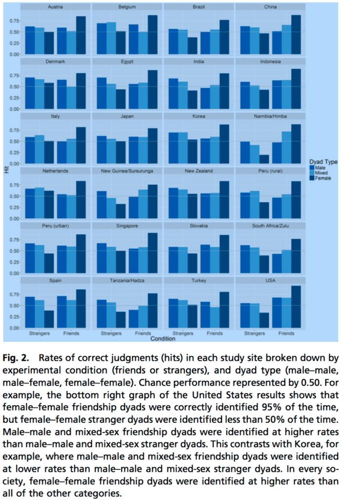
Hey—for the FF dyads they really do identify pairs of friends more accurately than chance for all 24 countries. How could that be???
Wait—I get it! For each dyad, participants had to guess Friend or Stranger. So what happened? Pairs of women were consistently guessed as Friends.
New headline: In 24 Countries, People Think Women Are More Friendly Than Men.
So, unless I”m missing something, the researchers made a classic statistical error: they evaluated a prediction by conditioning on the observed value. You can’t do that: you have to condition on the prediction.
Am I right here? Let’s check these intuitions by focusing on the U.S. and approximately reading the numbers off the graph. I divide each histogram bar height by 2, under the assumption that 50% of the true values are strangers and 50% are friends in each category.
Male and mixed dyads:
28% of the time it was a pair of strangers correctly identified as strangers
22% of the time it was a pair of strangers wrongly identified as friends
17% of the time it was a pair of friends wrongly identified as strangers
33% of the time it was a pair of friends correctly identified as friends
So, if you say Friend, there’s a 60% chance the person was actually a friend. If you say Stranger, there’s a 62% chance the person was actually a stranger. Pretty good!
Female dyads:
16% of the time it was a pair of strangers correctly identified as strangers
34% of the time it was a pair of strangers wrongly identified as friends
2% of the time it was a pair of friends wrongly identified as strangers
48% of the time it was a pair of friends correctly identified as friends
So, if you say Friend, there’s a 59% chance the person was actually a friend. If you say Stranger, there’s an 89% chance the person was actually a stranger. Pretty good too!
OK, so now I’m starting to think they’re on to something . . .
Yes there seem to be flaws in the analysis but, based on the data, it doesn’t seem to be just noise mining.
In particular, the statement from the paper, “Across all societies, listeners were able to distinguish pairs of colaughers who were friends from those who were strangers that had just met.”
Is this a big deal? I have no idea. The one thing I couldn’t figure out is how did they get the “brief, decontextualized instances of colaughter” from their recordings. If people are talking for awhile there could me more than one instance of laughing. Maybe strangers talking won’t laugh at all? I looked at the paper and the supplementary material but could find no instances where it said how they extracted the laughs. It’e probably there but I didn’t notice it. So I’ll reserve judgment on this one until I find out how the data were put together.
In any case, I wanted to share this, just so all of you can see my expectations confounded.
Typo, should be 60% in “So, if you say Friend, there’s a 06% chance”
Feel free to delete this comment.
Sometimes psychologists hope that two-alternative forced choice procedures would be “bias free”, but it is know, that this hope isn’t always guaranteed. I’d guess that this kind of task would be especially prone to bias, since the choices are so meaningful (not just eg. interval 1 or 2). And indeed they’ve calculated on the article that that was the case, but fastly skimming I couldn’t see any corrections done to the “raw” hit rates.
But that had me thinking, how about using a signal detection theoretical approach? The idea is to model the decisions about “friend or no friend” as latent gaussian distributions. When a pair of people who aren’t friends is presented colaughing, the certainty of them being friends varies randomly with mean 0 and varaince of 1; when a pair of people who are friends the certainty of them being varies randomly with mean 0 + d (and with variance 1 for simplicity’s sake). The more distinguishable friends are from non-friendies, the greater d will be.
Now, if the certainty exceeds some internal threshold, termed the criterion, the subject decides that the colaughterers are friends. This way, in theory and simplifying things, it should be possible to distinguish between genuine perceptual effects (the d) and shifts in this decisional criterion (ie. if people are more prone to answering “friends” when they here women colaughing.
Now, these can be calculated by having the hit and false alarm rates, and since Andrew kindly deduced them from the graph, I’ll use those.
For male and mixed pairs*:
(qnorm(0.33) – qnorm(0.22)) / sqrt(2)
sensitivity = 0.23
-((qnorm(0.33) + qnorm(0.22))) / sqrt(2)
criterion = 0.86
For female pairs:
(qnorm(0.48) – qnorm(0.34)) / sqrt(2)
sensitivity = 0.26
-((qnorm(0.48) + qnorm(0.34))) / sqrt(2)
criterion = 0.33
It would seem that there isn’t that much difference in the actual sensitivity, but people are more prone to answering “not friends” when male or mixed pairs are presented.
* formulae for calculating the measures are snatched from Kingdom & Prince: Psychophysics – A Practical Intoduction, p. 180.
I agree with you that SDT is a better tool for this than looking at hit rates alone. Though note that the graph gives the hit rates directly. Andrew divided by two to get the joint probabilities of each dyad type and response.
Using the hit and false alarm rates from the graph (i.e., multiplying the values you used by 2), using the formula d’ = z(hit)-z(false alarm), and expressing response bias as the signed distance from the crossover point of the two latent distributions (i.e., c = log(beta)/d’), I get d’ = .56 for males/mixed and d’ = 1.28 for females and c = -.13 for males/mixed and c = -1.1 for females.
So, I get larger magnitude differences in d’ and c, but reflecting the same general pattern.
Another quick note to point out that the task they used isn’t what I’ve typically seen described as a two-alternative forced choice task. Rather, on each trial of this study, a subject just saw/heard a colaughter stimulus, and s/he had to say if the two people were friends or strangers (i.e., it’s a friendship detection task). The important point here being that this task is not expected to be bias-free, whereas the 2AFC task is, at least relative to signal vs noise responses (but not necessarily with respect to stimulus position or interval or whatever). Note, too, that the sqrt(2) term is an adjustment to relate the 2AFC model to the detection model.
Strangers laughing together tend to be a coping mechanism to defuse a nervous situation of having just met. Friends laughing together tends to be less strategic.
My suggestion is that social scientists could use actors (e.g., improv comedians) to illustrate behaviors they are talking about in, say, accompanying videos. There are a lot of skilled actors who aren’t high paid stars but who can still conjure up a lot of different behaviors.
Or could you use old movies? There used to be a few great movies, most famously “It’s a Wonderful Life,” that had fallen out of copyright, but maybe there aren’t many anymore.