Paul Pudaite writes:
In the latest Journal of the American Statistical Association (September 2014, Vol. 109 No. 507), Andrew Harvey and Alessandra Luati published a paper [preprint here] — “Filtering With Heavy Tails” — featuring the phenomenon you had asked about (“…(non-Gaussian) models for which, as y gets larger, E(x|y) can actually go back toward zero.”).
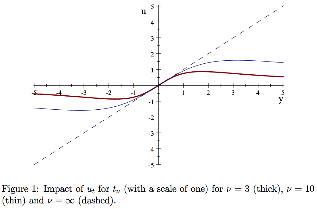
See their Figure 1, p. 1113:
They have a nice, brief discussion of the figure (also p. 1113):
The Gaussian response is the 45 degree line. For low degrees of freedom, observations that would be seen as outliers for a Gaussian distribution are far less influential. As |y|->Infinity, the response tends to zero.
They then note that:
Redescending M-estimators, which feature in the robustness literature, have the same property.
Unfortunately, they don’t provide any robustness literature references for redescending M-estimators. I guess it’s too well known!
(They do provide a reference for “the Huber M-estimator [which] has a Gaussian response until a certain point, whereupon it is constant”.)
The application in Harvey & Luati’s paper is railroad travel, so perhaps psychometricians still need to be alerted to these measurement error models.
I last posted on this topic in 2011.
> Unfortunately, they don’t provide any robustness literature references for redescending M-estimators. I guess it’s too well known!
Robust estimation methods used to figure prominently in my day-to-day work. (Not so much anymore.) I can’t recall ever establishing a “go to” set of references re redescending M-estimators. Re implementation, redescending estimators have stability issues, i.e., you need to ensure that your estimation algorithm precludes convergence on a “solution” where all data gets zero weight – a rookie mistake I made when I was a rookie.
I found this to be useful tutorial on M-estimators –
https://research.microsoft.com/en-us/um/people/zhang/inria/publis/tutorial-estim/node24.html
There’s a JASA paper on how inference for surprising data depends on the relative tail weight of the prior and model. I haven’t been able to find it in a brief search, but my (unreliable) recollection is that it’s not far from 1989.
The simplest example, which makes a nice math stat problem, is a Normal/Cauchy vs Cauchy/Normal. With a standard Normal prior and Cauchy data, if the observation is very large, the data are basically rejected and the posterior mode ends up near zero. With a standard Cauchy prior and Normal data, if the observation is very large, the prior is basically rejected and the posterior mode ends up near the data point.
The paper had a rather more general discussion of tail weight.
I think this is the paper I was recalling:
Outliers and Credence for Location Parameter Inference
Author(s): A. O’Hagan
Source: Journal of the American Statistical Association, Vol. 85, No. 409 (Mar., 1990), pp. 172-176
Stable URL: https://www.jstor.org/stable/2289540 .