Lu Zhang, Bob Carpenter, Aki Vehtari and I write:
We introduce Pathfinder, a variational method for approximately sampling from differentiable log densities. Starting from a random initialization, Pathfinder locates normal approximations to the target density along a quasi-Newton optimization path, with local covariance estimated using the inverse Hessian estimates produced by the optimizer. Pathfinder returns draws from the approximation with the lowest estimated Kullback-Leibler (KL) divergence to the true posterior. We evaluate Pathfinder on a wide range of posterior distributions, demonstrating that its approximate draws are better than those from automatic differentiation variational inference (ADVI) and comparable to those produced by short chains of dynamic Hamiltonian Monte Carlo (HMC), as measured by 1-Wasserstein distance. Compared to ADVI and short dynamic HMC runs, Pathfinder requires one to two orders of magnitude fewer log density and gradient evaluations, with greater reductions for more challenging posteriors. Importance resampling over multiple runs of Pathfinder improves the diversity of approximate draws, reducing 1-Wasserstein distance further and providing a measure of robustness to optimization failures on plateaus, saddle points, or in minor modes. The Monte Carlo KL-divergence estimates are embarrassingly parallelizable in the core Pathfinder algorithm, as are multiple runs in the resampling version, further increasing Pathfinder’s speed advantage with multiple cores.
The current title of the paper is actually “Pathfinder: Parallel quasi-Newton variational inference.” We didn’t say it in the above abstract, but our original motivation for Pathfinder was to get better starting points for Hamiltonian Monte Carlo, but then at some point it became clear that the way to do this is to get a variational approximation to the target distribution. I gave the above title to the blog post to draw attention to the idea that Pathfinder finds where to go.
In the world of Stan, we see three roles for Pathfinder: (1) getting a fast approximation (should be faster and more reliable than ADVI), (2) part of a revamped adaptation (warmup) phase, which again we hope will be faster and more reliable than what we have now, and (3) more effectively getting rid of minor modes. This is a cool paper (and I’m the least important of the four authors) and I’m really excited about the idea of having this in Stan and other probabilistic programming languages.
P.S. Bob provides further background:
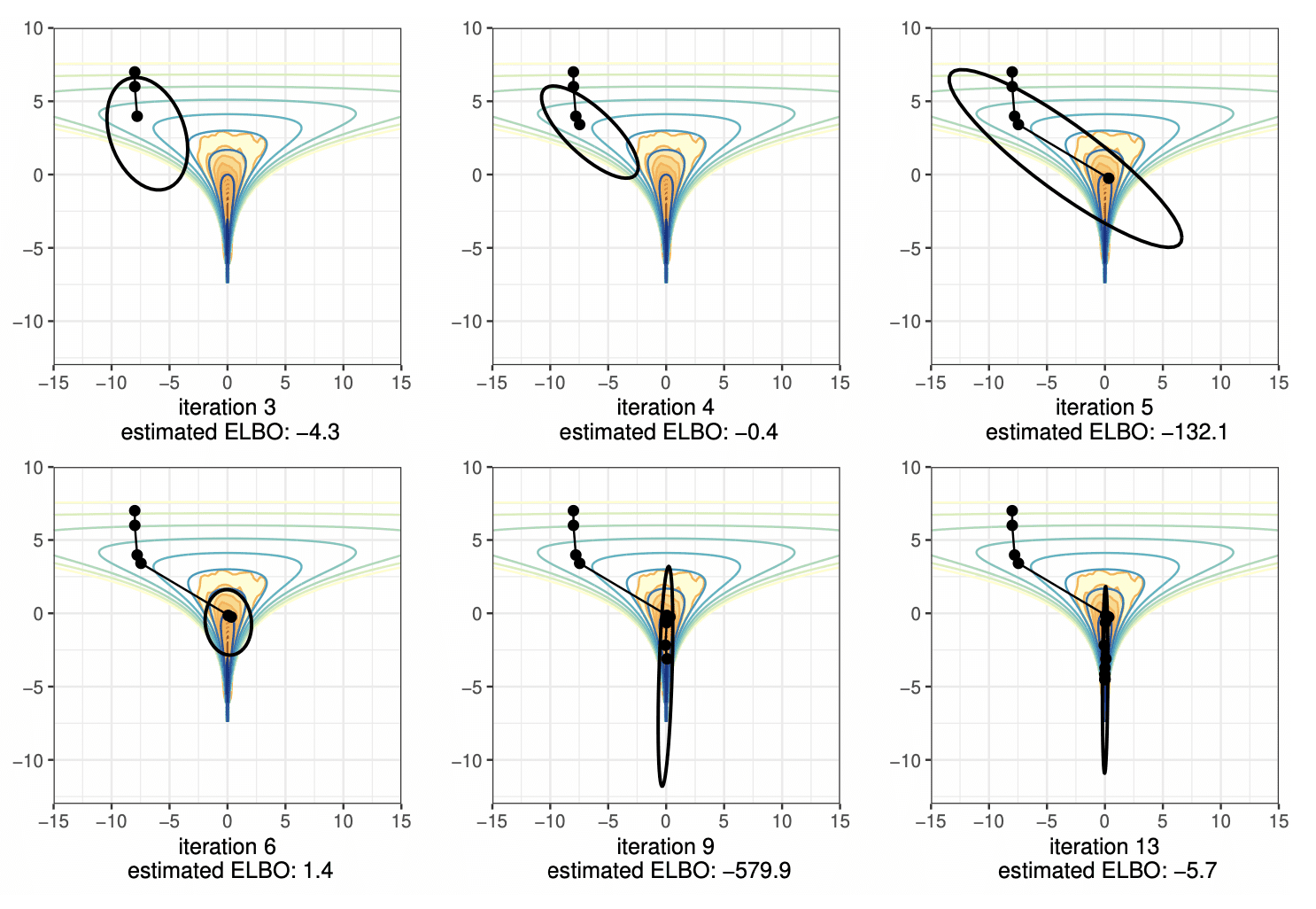
The original idea was based on the idea that the intermediate value theorem of calculus would guarantee that if we started with a random init in the tail and followed an optimization path, that path would have to go through the bulk of the probability mass on the way to the mode or pole (for example, hierarchical models don’t have modes because the density is unbounded). Here’s an ASCII art version of the diagram of what should happen,
*———[——–]———–> opt path
TAIL BODY HEADThe brackets pick out the region in the body of the distribution corresponding to reasonable posterior draws (see below for how we refined this idea). For instance, in a multivariate standard normal, this is a thin shell at a fixed radius from the mode at the origin.
We were at the same time playing around with the notion of typical set from information theory. The theorem around that is an asymptotic result for growing samples having a mean log density that approaches the entropy. We have been using it informally to denote the subset of the sample space where a sampler will draw samples. But that’s not quite what it is. Formally, the typical set with one draw is defined by sets of draws whose log density is within epsilon of the expected log density, i.e.,
Typical_epsilon = {theta : log p(theta | y) in E[log p(Theta | y)] +/- epsilon}.
This +/- epsilon business doesn’t work well when log p(Theta | y) is skewed, as it often is in applied problems. So instead we settled on the set of theta whose log densities fall the 99% central interval of log densities. That’s where 99% of our samples are drawn and should make a good target for initializing an MCMC sampler, our original goal.
Given an optimization path, we can evaluate the points in parallel to detect if they’re in the body of the distribution. If we start MCMC chains at those points, the ones in the tail should drift higher in density, the ones in the head should drift lower, whereas those in the body should bounce around. The only problem is that it’s hard to run MCMC on arbitrary densities robustly without a lot of adaptation, which is precisely what we were designing Pathfinder to avoid. Also, running MCMC is intrinsically serial. So next we considered evaluating the volume around a point and using density times volume as a proxy for being in the body of a distribution. We could use the low rank plus diagonal covariance approximation from the L-BFGS (quasi-Newton) optimizer to evaluate the volume. It worked better than MCMC and was very fast, but still failed in many cases. The final idea was to just evaluate the evidence lower bound (ELBO), equivalently KL-divergence from the approximation to the target density, at the normal approximation derived from L-BFGS at each point along the optimization path. That can also be done easily in parallel. It’s way more robust to run L-BFGS on the objective log p(theta | y) than it is to try to optimize the ELBO[normal(mu, Sigma) || log p(theta | y)] over mu and Sigma directly as ADVI does. We also don’t have the serialization bottleneck of ADVI where the evaluations of the ELBO need to be staged one after the other—all of our ELBO evals happen in parallel.
Along the way, we lost the original Pathfinder idea of finding a point in the optimization path in the body of the distribution. The point at which the best ELBO is located is often beyond the body of the distribution. For example, the best normal approximation for a multivariate normal is located at the mode.
After the basic idea worked, we found it getting trapped in local optima. The last idea was to run multiple optimization paths of Pathfinder in parallel, then importance resample the results. That essentially gives us a low-rank multivariate normal mixture approximation of a posterior, and that worked much better. Each Pathfinder instance runs in parallel, too, and the only serialization bottleneck is importance resampling, which is fast.
Next up, we’re going to try to tackle Phase II of Stan’s warmup. The question is whether its covariance estimates will be good enough to circumvent or at least shorten Phase II warmup. Ben Bales has already done a lot of work around this in his thesis, like parallelizing adaptation in Phase II. The final goal, of course, is robust, massively parallelizable MCMC. But even without parallelization, Pathfinder is way faster than ADVI or Stan’s Phase I warmup.
I think the third to last word of the second paragraph may need an ‘h’. were -> where
Wow—I appreciate that people are reading these posts so carefully!
I just went to write this post and see that Andrew beat me to it!
The original idea was based on the idea that the intermediate value theorem of calculus would guarantee that if we started with a random init in the tail and followed an optimization path, that path would have to go through the bulk of the probability mass on the way to the mode or pole (for example, hierarchical models don’t have modes because the density is unbounded). Here’s an ASCII art version of the diagram of what should happen,
*———[——–]———–> opt path
TAIL BODY HEAD
The brackets pick out the region in the body of the distribution corresponding to reasonable posterior draws (see below for how we refined this idea). For instance, in a multivariate standard normal, this is a thin shell at a fixed radius from the mode at the origin.
We were at the same time playing around with the notion of typical set from information theory. The theorem around that is an asymptotic result for growing samples having a mean log density that approaches the entropy. We have been using it informally to denote the subset of the sample space where a sampler will draw samples. But that’s not quite what it is. Formally, the typical set with one draw is defined by sets of draws whose log density is within epsilon of the expected log density, i.e.,
Typical_epsilon = {theta : log p(theta | y) in E[log p(Theta | y)] +/- epsilon}.
This +/- epsilon business doesn’t work well when log p(Theta | y) is skewed, as it often is in applied problems. So instead we settled on the set of theta whose log densities fall the 99% central interval of log densities. That’s where 99% of our samples are drawn and should make a good target for initializing an MCMC sampler, our original goal.
Given an optimization path, we can evaluate the points in parallel to detect if they’re in the body of the distribution. If we start MCMC chains at those points, the ones in the tail should drift higher in density, the ones in the head should drift lower, whereas those in the body should bounce around. The only problem is that it’s hard to run MCMC on arbitrary densities robustly without a lot of adaptation, which is precisely what we were designing Pathfinder to avoid. Also, running MCMC is intrinsically serial. So next we considered evaluating the volume around a point and using density times volume as a proxy for being in the body of a distribution. We could use the low rank plus diagonal covariance approximation from the L-BFGS (quasi-Newton) optimizer to evaluate the volume. It worked better than MCMC and was very fast, but still failed in many cases. The final idea was to just evaluate the evidence lower bound (ELBO), equivalently KL-divergence from the approximation to the target density, at the normal approximation derived from L-BFGS at each point along the optimization path. That can also be done easily in parallel. It’s way more robust to run L-BFGS on the objective log p(theta | y) than it is to try to optimize the ELBO[normal(mu, Sigma) || log p(theta | y)] over mu and Sigma directly as ADVI does. We also don’t have the serialization bottleneck of ADVI where the evaluations of the ELBO need to be staged one after the other—all of our ELBO evals happen in parallel.
Along the way, we lost the original Pathfinder idea of finding a point in the optimization path in the body of the distribution. The point at which the best ELBO is located is often beyond the body of the distribution. For example, the best normal approximation for a multivariate normal is located at the mode.
After the basic idea worked, we found it getting trapped in local optima. The last idea was to run multiple optimization paths of Pathfinder in parallel, then importance resample the results. That essentially gives us a low-rank multivariate normal mixture approximation of a posterior, and that worked much better. Each Pathfinder instance runs in parallel, too, and the only serialization bottleneck is importance resampling, which is fast.
Next up, we’re going to try to tackle Phase II of Stan’s warmup. The question is whether its covariance estimates will be good enough to circumvent or at least shorten Phase II warmup. Ben Bales has already done a lot of work around this in his thesis, like parallelizing adaptation in Phase II. The final goal, of course, is robust, massively parallelizable MCMC. But even without parallelization, Pathfinder is way faster than ADVI or Stan’s Phase I warmup.
P.S. Believe it or not, this was Lu’s first algorithms project! I can’t wait to see what she does for an encore. Most of the cool ideas in this project were hers and she also did all the hard coding work. Not to mention spelunking in old Fortran codes to figure out how L-BFGS really worked.
P.P.S. posteriordb was also a huge help in making this possible.
So with this it’s easier to get to sampling — do you think this lessens the model-diagnosing usefulness of multi-chain MCMC in any practical way?
I’m guessing since this isn’t changing the MCMC that comes after and models that sampled badly cause of unidentified parameters or bugs or whatnot are still going to sample badly.
I like that this got baked into the pie:
> The last idea was to run multiple optimization paths of Pathfinder in parallel, then importance resample the results.
The last time I hit multiple mode that made mixing bad was Dawid-Skene and in that case I changed my priors to work around it, so I don’t really mind if this happens more automatically for me in the future, but maybe I’m not being creative enough to think about another problem.
No, I think we still want to run multi-chain diagnostics. The importance sampling can help mitigate some of the problems, but it’s not guaranteed to solve them or we would’ve included a theorem to that effect.
We don’t plan to change how HMC works. But we do hope to be able to replace the first one or two stages of warmup as we currently do them in Stan with Pathfinder.
The Dawid-Skene model was my gateway to Bayes. I was working in NLP and had lots of data sets with crowdsourced labels. Andrew and Jennifer Hill helped me formulate a model that turned out to be identical to the Dawid-Skene model on the logit scale with hierarchical priors. If there are only two categories, you can avoid the antagonistic/non-cooperative mode by requiring sensitivity > (1 – specificity). It’s a little trickier with K categories, especially when they can be informative ordinal things with high error.
Oh oh so all this is still done per-chain. Makes sense.
The single-path version of Pathfinder works on a single optimization path. The multi-path version importance resamples approximate draws from multiple runs of single-path Pathfinder (Lu figured out how to efficiently evaluate proper mixture importance weights, and I think Aki found some literature on the problem that’s cited in the paper).
The plan is then to take approximate draws from Pathfinder and use those to initialize multiple MCMC chains. Those MCMC chains should still be checked for mixing. The obstacle there is if we only run each MCMC chain for a very short number of draws, statistics like R-hat will be too high variance. So I guess we need to add multiple short-chain diagnostics to our to-do list. Shooting from the hip, I’m thinking we might be able to get away with dividing the N short chains into M groups (M << N) and compare the M groups using R-hat. Nothing in basic R-hat relies on the order of the draws; split R-hat, on the other hand, compares the first half of a chain with the second half.
> I’m thinking we might be able to get away with dividing the N short chains into M groups (M << N)
Oh huh, yeah I could see where this would work. Feels like some sort of cross-validatey thing, but I don't have a feel for how Rhat might fail so not sure what assumptions are appropriate.
As someone who is still learning about this whole space, I’m curious as to understanding what “robust, massively parallelizable MCMC” looks like in practice and how it squares with the reality that “running MCMC is intrinsically serial”.
Is the idea that by significantly speeding up the warmup phases, we get more benefits from running many chains at once since we no longer have to pay the (effectively) serial cost of performing warmup across all chains?
Yes, that’s our thinking. Imagine running 100 or even 1000 chains to get 1 draw each. I was originally inspired by Matt Hoffman’s talks and paper on this, which we cite heavily in the paper. The main bottleneck is in converging and adapting. If we could converge and adapt instantly, then we could get 100 or 1000 draws in parallel in a time bounded by autocorrelation time.
exciting work! Thanks for the response.
We’ve had discussions like this in the past, for example: https://discourse.mc-stan.org/t/the-typical-set-and-its-relevance-to-bayesian-computation/17174/19
Where it sounds like you were in the starting stages of this work described here.
In general, if {x_i} is some “decent approximate sample from a distribution q(x)” then {T(x_i,n)} where T is an MCMC transition process run for n steps is a sample “closer to p(x)” the target distribution of T. As n goes to infinity, obviously it’s now a perfect sample from p(x).
If you can get some initial sample that’s “pretty good” then you can make n small… and also T can be a fairly simple markov chain (say, just a diffusive MH rather than HMC)
So, if you can start from some kind of ok initial ensemble sample, you can run a simple diffusive monte carlo on each sample point for a few iterations, and get an even better approximation… you can repeat this and check for convergence of the ensemble…
Perhaps Pathfinder provides this good starting point, and something as simple as diffusive metropolis can “finish it”?
Stone-Soup! Or in some versions “Nail-soup”.
Every fancy global optimization scheme that is supposed to get you to the “best” finishing value has to either [a] test a dense grid of starting values; or [b] somehow find a starting value which is itself pretty near “best”.
In my experience with enough work one ends up with a method that generates some reasonable starting value; the scheme then chugs away and reports the sought-after optimum; the conference-paper is published.
But on retrospection, looking at the code in the rear-view mirror, I always see: “Stone soup!”. A great complex preparation setup so that the “sophisticated” method could get to work (and arrive at the right answer).
Fucking incredible paper. Not just for the main idea, but the clarity of the refreshers on L-BGFS and related inverse Hessian covariance estimators too. I love the triple presentation of the tricky computational algorithms. Pseudocode + captioned explanations of reasoning for steps + a high level text descriptions for reinforcement.
I remember a few years back an idea that got kicked around and ruled out was initializing HMC with the MAP estimate, the problem being that the mode is usually far from the typical set in higher dimensions. Is that not true for the ELBO maximizing approximation? More specifically, is there a more formal treatment of this passage and why it works?
Thanks. I pushed very hard for getting complete pseudocode. Figuring out all those L-BFGS details was all Lu. She was literally digging through old Fortran code to see what they actually did. Extensive captioning is Andrew’s thing.
A big problem with MAP estimates is that they don’t exist for hierarchical models, simple mixtures, etc. because the log density is not bounded. For example, in a hierarchical model
We get unbounded log density as sigma -> 0 and as alpha[n] -> 0. In a mixture, if we put one observation in a mixture component with zero variance we get infinite log density (or as MacKay says in his great book, “EM goes boom.”).
The normal approximation found by Pathfinder is often centered at the mode, but then we take draws from it, not the mode itself to initialize. For example, PyMC3 lets you initialize with either the ADVI mean or a draw from the ADVI approximation. At one point, Lu had evaluations for using the variational mean for inference, but they wound up on the cutting room floor like another half dozen diagrams we had.
In hard applied problems, I find myself sometimes writing a model that I can fit with max likelihood and often using those points to initialize MCMC. For example, if you get replace hierarchical priors with fixed priors, you don’t have the infinite log density problem and you can estimate initials for hierarchical variance with the variance of the MLE fits. We’re trying to talk about moves like this in our Workflow paper and book, but we’re also trying to fight it sprawling out of control.
From the paper:
If I understand correctly, the pathfinder algorithm makes some assumptions about the posterior (eg, unimodal), and thus finds the best parameter much faster… when those assumptions hold. This seems to be just like automating your max likelihood initialization. Both are throwing more assumptions into the model.
Is the trade-off vs. a random initialization with normal MCMC burn-in that you are less likely to notice your model is misspecified?
If not that, there must be some trade-off(s) for making additional assumptions. What are they? Sorry if I missed it in the paper.
I thought it was probably a little bit more robust to multimodality than regular HMC
1. It optimizes over bayesian log probability rather than max likelihood
2. It doesn’t find one initialization at the maximum, but rather sets off a bunch of approximations at many points along the path from the start to the optimum and picks the best one. So even if the MAP diverges it can find a best approximation somewhere between the starting point and the singularity.
3. Multimodality can be accommodated by setting off the algorithm multiple times with random initialization. So it should be fairly robust as long as the random initialization has good enough coverage over the plausible region of the posterior, you’re running enough copies of the algorithm, and the posterior can be approximated by a finite gaussian mixture.
The trade off seems like finite gaussian approximation error
Oh, this is a clearer reply than mine. Thank you so much!
If that really is it, then this is just great. However, I suspect it is similar to cherry-picking initial values (which is a common dark art, alongside playing with priors and other hyperparameters until it “works”). Obviously, doing that introduces the possibility the chains converge misleadingly. I.e., when you initialize to a high density region they may not leave it to explore other modes.
I think everyone agrees that the choice of initialization is not supposed to affect the final distribution, it should only affect how fast you get convergence.
I’m just not convinced this method avoids introducing assumptions about the posterior that aren’t included in the actual model, where they belong. This runs the risk of forcing the posterior to meet these assumptions.
It seems like a step forward in that it is actually more transparent than the current practice of speeding up (or forcing) convergence by cherry-picking the initial values. Still, if the model is incorrectly specified then we do not want the chains to converge. That is our signal to fix the model.
Anon:
I used to have that attitude too—the idea that choosing inits is a sort of cheating—but I no longer believe that. I agree that ideally the result of the algorithm won’t depend on inits, but we don’t always live in an ideal world. It’s common for models to have unimportant minor modes;; see for example the planetary motion example in section 11 of our workflow paper.
Saying that inits shouldn’t matter is kinda like saying that algorithms should be closed form and not iterative. If that happens, great, but if not, we should be realistic that inits can matter.
There are two cases to be discussed here
1. pathfinder as approximate bayes
2. pathfinder as fast initialization for HMC
It sounds like you’re worried about in the second case, pathfinder skipping over meaningful structure, then HMC spending the whole chain in a small region about the main mode. I’m no expert, but I feel like because the pathfinder initialization is itself random uniform and then random draws are taken for the HMC initialization it *should* find most of the important high-mass regions, if the pathfinder init gets good coverage. I’m guessing that the last bit may not be satisfied in high dimensions with especially weird posterior geometry with a finite number of pathfinder runs due to concentration of measure.
People won’t pay attention to anything not explicitly stated in the model. Ignoring this will result in new ways of p-hacking.
What you call “especially weird” is basically every real world application. In fact, can you name an example where this is not the case?
This is just not true. In the paper under discussion many real world datasets and problems are given with a well-understood reference posterior which do not exhibit the described pathologies with pathfinder.
I guess there are probably some real world problems without pathologies, but then you probably don’t need pathfinder for them. In the vast majority of problems I’ve tackled, there’s some difficulty in fitting. I feel lucky when I can start Stan and get back 2000 samples in less than an hour and they seem to be converged.
Daniel:
Pathfinder’s not just for when it’s “needed”; the plan is to set it up by default so it can speed things up on the easy problems too. This is similar to how in Regression and Other Stories we use Bayes for everything, rather than holding it in reserve for when it’s needed.
Agreed, it shouldn’t hurt to use something like Pathfinder to start your chains, but when the problem is complex enough, if you start your chains without it you’ll spend hours getting into the high probability region and you’ll never be able to debug your model. This was definitely my experience in 2017 when I tried to model simultaneously every county in the country base living expenses as a function of family composition. Just getting it past initialization was excruciating.
Daniel:
Yup! And that workflow was especially a problem given our attitude of being too proud to think hard about inits.
Somebody:
Real world application != real world dataset. I didn’t look into the datasets, but I would bet those have been chosen via a process of trial and error over the years. You won’t get published (or even try) if you can’t make your algorithm perform to some minimal standard.
Daniel Lakeland:
This is what I mean. It is very common. That is a signal to fix your model. Or maybe you simply don’t have the right type of data available so the model is underdetermined. In either case, we should not take the model output seriously.
https://en.wikipedia.org/wiki/Underdetermination
I guess in the end it is the same as anything else, use your method to make a prediction about future data and see how well it does.
Actually in my case the model was extremely precisely identified, so that it had to sample in a very very tight region of space using extremely small timesteps and the slightest step outside the sharply identified region caused divergence. The model was fabulous, it was the sampling that was problematic ;-)
So you generated fake data from the exact same model, so we know the model is correctly specified, then when you try to fit it you still saw this problem?
It’s not really about correctness, but rather just the difficulty of sampling when you need to slot into a very deep potential well starting from a random point nowhere near that slotted trench.
For example, suppose you have 1000 genes where you’ve measured counts in an RNAseq experiment. The counts can range from on the order of around 10 to on the order of 300000 but they tend to be fairly consistent, so across different experiments within 10% of each other. The “initalization problem” then is to find a vector of 1000 numbers like:
3,7,201,39338,13,92,770,50515,393412,10,….
and in order for the problem to start sampling well, you have to be within 10% of the proper number in **every** one of the 1000 dimensions
Now suppose the standard method to “initialize” is to just choose a number between 1 and 10 for each dimension (or something like that).
Getting to the right starting place is ridiculously computationally obnoxious, because you’re doing HMC and you’re in a regime where it’s got tremendous potential energy because you’re VERY far from the right answer in some dimensions, so it’s like a nuclear bomb at detonation, the equations tell you to shoot off into the stratosphere, and the step size that makes sense is tiny tiny tiny, so you have to do a bazillion calculations just to get to the point where eventually you’re floating around calmly bobbing on the wind-blown waves in a swimming pool.
That’s the basic flavor. Even if the sampling problem isn’t hard once you get to the right region and have tuned the proper step size and etc… starting from some stupid random point can easily take a bazillion calculations to find the right sampling region.
This sounds like the model is missing something to me. There is something categorically different between people with a +/- 10% value of 300k vs 10. If that is missing from the model then you get the type of issue you describe.
This is just a measurement error model for 1000 simultaneous measurements that all have vastly different scales. Imagine you’re measuring cells from some tissue, you’re measuring the number of mRNAs for each of 1000 different genes. You have 20 different sample cells from the tissue.
It’s totally normal for some genes to not be expressed much at all, and other genes to be expressed extremely highly. Hence some genes have 10 copies of mRNA, other genes have 390,000 copies, other genes have 40,000 copies others have 300…
The model is well specified, and from one cell to another the differences are only 10% for each gene… but you can’t start sampling until you find the right region in space that specifies “what these cells are generally like”. It’s a point in 1000 dimensional space
Eg, use: https://en.wikipedia.org/wiki/Dirichlet_process
Yes, you get the same problem though. Starting from a point far away from the right answer, you can’t get to the right answer and sample efficiently without some kind of initialization procedure that does a good job. This is precisely because the right answer is tightly identified and hence from any “random” initialization point, you’re pretty much guaranteed to be in the “nuclear bomb” initial conditions.
Think of it like this… you’ve got a great skate park for skateboarders. They have little ramps and stairs and half pipes and all that stuff. The sampling procedure you should be doing is “skating around in the park”… The only problem is the skate park is in LA and you’re in NYC, and furthermore the skate park walls extend all the way to NYC and are enormously vertical so that although you’re still technically in the skate park in NYC you’re up at the altitude of the moon. So your job is to drop into this skate park at the altitude of the moon, bomb down the side of this basically vertical wall at eventually Mach 9500 in a earth-shattering asteroid collision type situation… so that you can eventually skate around calmly at 5-11 mph within 2m of the surface of the LA skate park.
it’d really be much better to get on an airplane, fly to LA and drive to the skate park and drop in to the half pipe wall at 2m high.
+1 for sports analogy
+1 for NY/LA connection
If you initialize to somewhere with no gradient to follow this is what MCMC is supposed to do until it finds one though (which can take forever). That is why no one does this if they can help it. I mean, why would you start out somewhere your model says is impossible?
The trade-off is you are introducing assumptions about the posterior into the initialization method. Those assumptions belong in the model where everyone will see them, because it can lead to a falsely confident picture of the posterior.
Until someone solves P = NP in the affirmative, we’re not going to have algorithms that can sample from combinatorially intractable posteriors like 3D Ising models. And just to be clear, we’re not claiming to solve P = NP in the affirmative.
We were very clear in the paper that Pathfinder is a form of approximate inference. Even if we didn’t have to worry about floating point, there are latent biases due to initialization which we discuss at length in the paper. It’s the exact same problem that MCMC, optimization, and other forms of variational inference have from initialization.
Stan’s documentation does not recommend cherry-picking initial values with MCMC precisely because it can lead to bias. Stan throws lots of warnings in situations where R-hat fails or estimated head or tail ESS is too low. Even when R-hat and ESS are consistent with convergence, we urge caution because they are only necessary conditions for convergence, not sufficient. That’s why we encourage posterior predictive checks and cross-validation or held-out evaluation. Stan also warns users in cases where there are divergences in the Hamiltonian simulation, which is usually caused by an ill-conditioned posterior. That often happens in high curvature regions of hierarchical models, typically biasing posterior estimates away from low hierarchical variance regions. That’s why we throw warnings—to alert the user there may be a problem, not so they can throw away chains.
As a methodological aside, we often tweak priors because we have more information than we initially encoded. For example, if I try to fit the Dawid-Skene crowdsourcing model to binary data, there are two modes, one adversarial and one cooperative. When we realize there’s an adversarial mode, we can constrain it away by requiring sensitivity > (1 – specificity) when we know we are dealing with cooperative coders. Are we worried we’ll misfit the model? No, because if there is an adversarial coder among the cooperative ones, it’ll show up in their estimated sensitivities and specifies being on the boundaries. Researchers don’t ask Nature for a model to bring to data. It’s an iterative process of engineering in models where we care about the predictive power. We typically don’t compute p-values or Bayes factors, so p-hacking per se isn’t an issue. We often have grand scientific ideas about modeling, but which particular model we can use depends on how much data we have and how good our sampler. That turns out to be an empirical question. Sometimes we even have to go get more data to have more informative priors—this comes up all the time in bio modeling, where we might do a meta-analysis to establish priors for our current analysis.
The case we’re mostly excited about for Pathfinder is where the posterior is so poorly conditioned that it’s hard to get started with HMC. Like the case Daniel Lakeland mentioned. Will we have guarantees? Afraid not. Will it work faster and more reliably than what we currently do? We hope so.
@Bob
All I’m saying is there must be some substantial tradeoff involved to get 1-2 orders of magnitude speedup here, and I don’t think it is limited to sampling error. It may only show up in edge cases where some assumption is heavily violated, but when it shows up it could be nasty and lead to very misleading conclusions.
That is already the status quo, and if you are going to add assumptions to the initialization why not do it right. This method looks like a very useful improvement to me and I would use it.
Why must there be a substantial tradeoff? If you’re using bubblesort to sort a billion numbers and someone comes along and changes it to quicksort, you’ll get many orders of magnitude of speedup with zero downside. I suspect this is similar. Basically optimization routines don’t have divergences, don’t require tiny timestamps to be stable, and etc. So they are a good way to find where to start sampling. This just takes it one step further and starts approximating the region around the step points.
I’ve never implemented bubblesort or quicksort, but usually when I code it involves first writing a slow and ugly ram hungry prototype. Then later I clean it up and optimize it.
So the tradeoff could be that it is easier to implement and understand bubblesort, or maybe it could be ram requirements?
Hi Anoneuoid.
The problem of Pathfinder for the ovarian example we show in the paper is that when initializing with points from uniform(-2, 2), all optimization paths converge to the mode around the origin. So the optimization paths cannot provide information to approximate posterior around the high probability mass regions. If the optimization paths explore the high probability mass regions as shown in Figure 24b, Pathfinder will give reasonable results. So if there must be an additional assumption, I think the assumption should be that the optimization paths need to explore high probability mass regions. For difficult posteriors with minor modes, bad initials can violate this assumption. It is true that this assumption can be hard to be satisfied for some difficult posteriors as we discussed in Section 3.3. But at the same time we show that pathfinder works well for a wide variety of models. Our follow-up researches will focus more on those difficult posteriors. And I would like to emphasize that Pathfinder uses normal approximations to generate approximate draws. So it is different from automating max likelihood initialization, which only provides a single point.
Thanks, but why exactly would it miss minor nodes and fail on flat posteriors? There is something being assumed about the posterior here. Is it that the algorithm assumes the posterior is a mixture of < n normal distributions, where n is the number of pathfinder runs?
As mentioned above, I am more concerned with getting a false picture of posteriors a misspecified model cannot fit rather than lack of convergence here.
Thank you so much for the post! The paper cannot be there without you. ^_^
> The final idea was to just evaluate the evidence lower bound (ELBO), equivalently KL-divergence from the approximation to the target density, at the normal approximation derived from L-BFGS at each point along the optimization path.
Wait so does this mean that in these evaluations pathfinder is better at VI than ADVI?
Like in any of the experiments if you’d initialized the ADVI at the pathfinder approx then the ADVI would just stay there (on its own it would just be worse)?
Yes, it’s better at VI than ADVI on most of the problems we evaluated.
We believe that come from two sources: (a) using low-rank covariance, and (b) the problems ADVI faces using SGD directly on the ELBO. ADVI as implemented in Stan will have ELBO values bounce around in later iterations due to the stochastic gradient—you’ll see that along with warnings if you run for enough iterations with a tight enough convergence tolerance.
For (b), Sifun Liu and Art Owen have a paper Quasi-Newton Quasi-Monte Carlo for variational Bayes, where they use QMC to tackle the high variance, which lets them use L-BFGS on the ELBO optimization.
For (a), others have looked at improving ADVI to use low-rank approximations. I thought we cited one of those in the paper, but now I can’t find it. We should be citing it! I also found this paper by Tomczak et al., Efficient Low Rank Gaussian Variational Inference for Neural Networks.
Have you considered ramping up hype before dropping bangers like this? I can’t be waking up in the morning, thinking it’s a day like any other, and finding this with no warning
Somebody:
Well, I did think it was important enough to post without the usual 6-month lag.
How can I upvote these comment threads? :D
Could you please share the paper.
Link is at beginning of above post.
Thank you so much for the post! ^_^
Very nice, and I see a nice theme in you guys really leveraging matrix decomposition in statistical computation. Any idea on whether other approximation families such as normal-inverse gamma help – for instance for the horseshoe application mentioned in the paper. The need to use other approximations in large-scale mean-scale-ish ADVI was the reason I initially stopped using Stan for some problems but this work makes me want to start using Stan more.
Section II says: “This section describes the Pathfinder algorithm for generating approximate draws from a differentiable target density known only up to a normalizing constant.” However, it seems that the description of the algorithm assumes a normalized target density. (In particular Figure 9, but I don’t think that it makes a substantial difference.)
Figure 9? Do you mean the ELBO estimation? Whether p() is normalized or not doesn’t matter since we only care about which approximation maximizes the estimated ELBO. An unnormalized target density will cause a shift in the ELBO estimation, but for the same model, the shifts in the ELBO estimates will be the same.
Whether p is normalized or not does matter for the correctness of those formulas. I agree that the missing factor doesn’t change the result of the “arg min” operator.
Oh, I see. So you mean the description of the algorithm is a little bit misleading. Thank you for the comment.
Looking at it again I’ve realized that I was wrong.
Fig. 9 doesn’t assume that p is the (normalized) target density p(phi|y).
Quite the contrary: it stands for the joint density p(phi, y) as in formula II.5.