My enemies are all too familiar. They’re the ones who used to call me friend – Jawbreaker
Well I am back from Australia where I gave a whole pile of talks and drank more coffee than is probably a good idea. So I’m pretty jetlagged and I’m supposed to be writing my tenure packet, so obviously I’m going to write a long-ish blog post about a paper that we’ve done on survey estimation that just appeared on arXiv. We, in this particular context, is my stellar grad student Alex Gao, the always stunning Lauren Kennedy, the eternally fabulous Andrew Gelman, and me.
What is our situation?
When data is a representative sample from the population of interest, life is peachy. Tragically, this never happens.
Maybe a less exciting way to say that would be that your sample is representative of a population, but it might not be an interesting population. An example of this would be a psychology experiment where the population is mostly psychology undergraduates at the PI’s university. The data can make reasonable conclusions about this population (assuming sufficient sample size and decent design etc), but this may not be a particularly interesting population for people outside of the PI’s lab. Lauren and Andrew have a really great paper about this!
It’s also possible that the population that is being represented by the data is difficult to quantify. For instance, what is the population that an opt-in online survey generalizes to?
Moreover, it’s very possible that the strata of the population have been unevenly sampled on purpose. Why would someone visit such violence upon their statistical inference? There are many many reasons, but one of the big one is ensuring that you get enough samples from a rare population that’s of particular interest to the study. Even though there are good reasons to do this, it can still bork your statistical analysis.
All and all, dealing with non-representative data is a difficult thing and it will surprise exactly no one to hear that there are a whole pile of approaches that have been proposed from the middle of last century onwards.
Maybe we can weight it
Maybe the simplest method for dealing with non-representative data is to use sample weights. The purest form of this idea occurs when the population is stratified into $latex J$ subgroups of interest and data is drawn independently at random from the $latex j$th population with probability $latex \pi_j$. From this data it is easy to compute the sample average for each subgroup, which we will call $latex \bar{y}_j$. But how do we get an estimate of the population average from this?
Well just taking the average of the averages probably won’t work–if one of the subgroups has a different average from the others it’s going to give you the wrong answer. The correct answer, aka the one that gives an unbiased estimate of the mean, was derived by Horvitz and Thompson in the early 1950s. To get an unbiased estimate of the mean you need to use the subgroup means and the sampling probabilities. The Horvitz-Thompson estimator has the form
$latex \frac{1}{J}\sum_{j=1}^J\frac{\bar{y}_j}{\pi_j}$.
Now, it is a truth universally acknowledged, if perhaps not universally understood, that unbiasedness is really only a meaningful thing if a lot of other things are going very well in your inference. In this case, it really only holds if the data was sampled from the population with the given probabilities. Most of the time that doesn’t really happen. One of the problems is non-response bias, which (as you can maybe infer from the name) is the bias induced by non-response.
(There are ways through this, like raking, but I’m not going to talk about those today).
Poststratification: flipping the problem on its head
One way to think about poststratification is that instead of making assumptions about how the observed sample was produced from the population, we make assumptions about how the observed sample can be used to reconstruct the rest of the population. We then use this reconstructed population to estimate the population quantities of interest (like the population mean).
The advantage of this viewpoint is that we are very good at prediction. It is one of the fundamental problems in statistics (and machine learning because why not). This viewpoint also suggests that our target may not necessarily be unbiasedness but rather good prediction of the population. It also suggests that, if we can stomach a little bias, we can get much tighter estimates of the population quantity than survey weights can give. That is, we can trade of bias against variance!
Of course, anyone who tells you they’re doing assumption free inference is a dirty liar, and the fewer assumptions we have the more desperately we cling to them. (Beware the almost assumption-free inference. There be monsters!) So let’s talk about the two giant assumptions that we are going to make in order for this to work.
Giant assumption 1: We know the composition of our population. In order to reconstruct the population from the sample, we need to know how many people or things should be in each subgroup. This means that we are restricted in how we can stratify the population. For surveys of people, we typically build out our population information from census data, as well as from smaller official surveys like the American Community Survey (for estimation things about the US! The ACS is less useful in Belgium.). (This assumption can be relaxed somewhat by clever people like Lauren and Andrew, but poststratifying to a variable that isn’t known in the population is definitely an adanced skill.)
Giant assumption 2: The people who didn’t answer the survey are like the people who did answer the survey. There are a few ways to formalize this, but one that is clear for me is that we need two things. First, that the people who were asked to participate in the survey in subgroup j is a random sample of subgroup j. The second thing we need is that the people who actually answered the survey in subgroup j is a random sample of the people who were asked. These sort of missing at random or missing completely at random or ignorability assumptions are pretty much impossible to verify in practice. There are various clever things you can do to relax some of them (e.g. throw a hand full of salt over your left shoulder and whisper “causality” into a mouldy tube sock found under a teenage boy’s bed), but for the most part this is the assumption that we are making.
A thing that I hadn’t really appreciated until recently is that this also gives us some way to do model assessment and checking. There are two ways we can do this. Firstly we can treat the observed data as the full population and fit our model to a random subsample and use that to assess the fit by estimating the population quantity of interest (like the mean). The second method is to assess how well the prediction works on left out data in each subgroup. This is useful because poststratification explicitly estimates the response in the unobserved population, so how good the predictions are (in each subgroup!) is a good thing to know!
This means that tools like LOO-CV are still useful, although rather than looking at a global LOO-elpd score, it would be more useful to look at it for each unique combination of stratifying variables. That said, we have a lot more work to do on model choice for survey data.
So if we have a way to predict the responses for the unobserved members of the population, we make estimates based on non-representative samples. So how do we do this prediction.
Enter Mister P
Mister P (or MRP) is a grand old dame. Since Andrew and Thomas Little introduced it in the mid-90s, a whole lot of hay has been made from the technique. It stands for Multilevel Regression and Poststratification and it kinda does what it says on the box.
It uses multilevel regression to predict what unobserved data in each subgroup would look like, and then uses poststratification to fill in the rest of the population values and make predictions about the quantities of interest.
(This is a touch misleading. What it does is estimate the distribution of each subgroup mean and then uses poststratification to turn these into an estimate the distribution of the mean for the whole population. Mathematically it’s the same thing, but it’s much more convenient than filling in each response in the population.)
And there is scads of literature suggesting that this approach works very well. Especially if the multilevel structure and the group-level predictors are chosen well.
But no method is perfect and in our paper we launch at one possible corner of the framework that can be improved. In particular, we look at the effect that using structured priors within the multilevel regression will have on the poststratified estimates. These changes turn out not to massively change whole population quantities, but can greatly improve the estimates within subpopulations.
What are the challenges with using multilevel regression in this context?
The standard formulation of Mister P treats each stratifying variable the same (allowing for a varying intercept and maybe some group-specific effects). But maybe not all stratifying variables are created equal. (But all stratifying variables will be discrete because it is not the season for suffering. November is the season for suffering.)
Demographic variables like gender or race/ethnicity have a number of levels that are more or less exchangeable. Exchangeability has a technical definition, but one way to think about it is that a priori we think that the size of the effect of a particular gender on the response has the same distribution as the size of the effect of another gender on the response (perhaps after conditioning on some things).
From a modelling perspective, we can codify this as making the effect of each level of the demographic variable a different independent draw from the same normal distribution.
In this setup, information is shared between different levels of the demographic variable because we don’t know what the mean and standard deviation of the normal distribution will be. These parameters are (roughly) estimated using information from the overall effect of that variable (total pooling) and from the variability of the effects estimated independently for each group (no pooling).
But this doesn’t necessarily make sense for every type of demographic variable. One example that we used in the paper is age, where it may make more sense to pool information more strongly from nearby age groups than from distant age groups. A different example would be something like state, where it may make sense to pool information from nearby states rather from the whole country.
We can incorporate this type of structured pooling using what we call structured priors in the multilevel model. Structured priors are everywhere: Gaussian processes, time series models (like AR(1) models), conditional autogregressive (CAR) models, random walk priors, and smoothing splines are all commonly used examples.
But just because you can do something doesn’t mean you should. This leads to the question that inspired this work:
When do structured priors help MRP?
Structured priors typically lead to more complex models than the iid varying intercept model that a standard application of the MRP methodology uses. This extra complexity means that our we have more space to achieve our goal of predicting the unobserved survey responses.
But as the great sages say: with low power comes great responsibility.
If the sample size is small or if the priors are set wrong, this extra flexibility can lead to high-variance predictions and will lead to worse estimation of the quantities of interest. So we need to be careful.
As much as I want it to, this isn’t going to turn into a(nother) blog post about priors. But it’s worth thinking about. I’ve written about it at length before and will write about it at length again. (Also there’s the wiki!)
But to get back to the question, the answer depends on how we want to pool information. In a standard multilevel model, we augment the information within subgroup with the whole population information. For instance, if we are estimating a mean and we have one varying intercept, it’s a tedious algebra exercise to show that
$latex \mathbb{E}(\mu_j \mid y)=\approx\frac{\frac{n_j}{\sigma^2} \bar{y}_j+\frac{1}{\tau^2}\bar{y}}{\frac{n_j}{\sigma^2}+\frac{1}{\tau^2}}$,
so we’ve borrowed some extra information from the raw mean of the data $latex \bar{y}$ to augment the local means $latex \bar{y}_j$ when they don’t have enough information.
But if our population is severely unbalanced and the different groups have vastly different different responses, this type of pooling may not be appropriate.
A canny ready might say “well what if we put weights in so we can shrink to a better estimate of the population mean?”. Well that turns out to be very difficult.
Everybody needs good neighbours (especially when millennials don’t answer the phone)
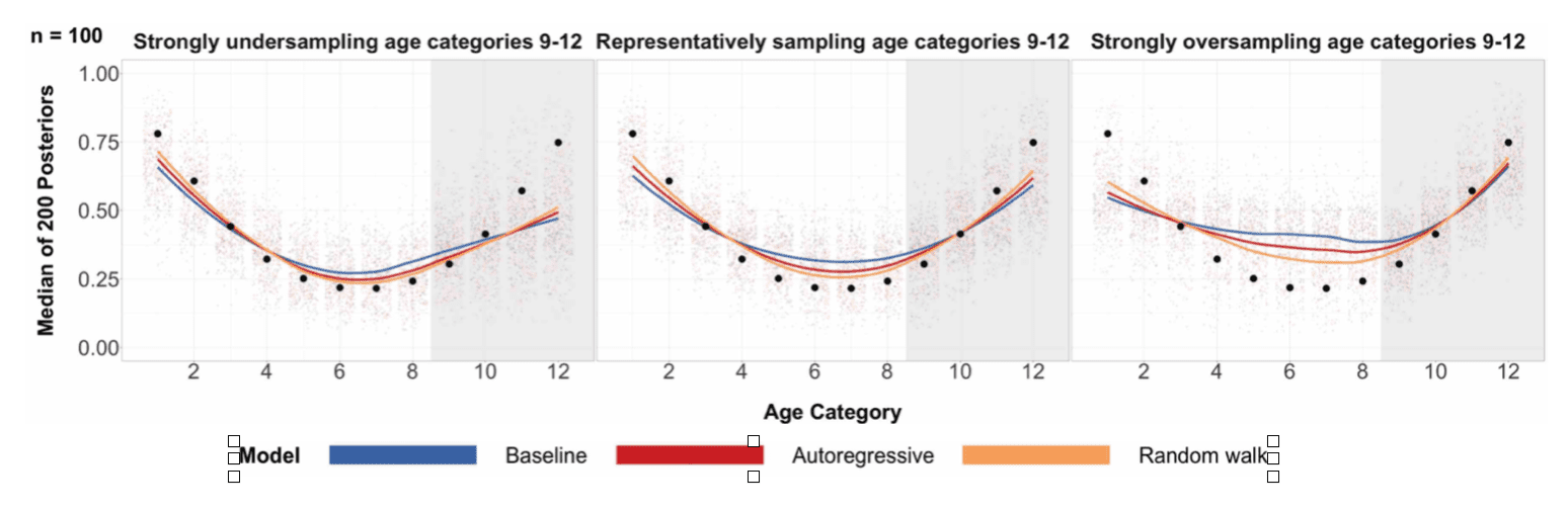
The solution we went with was to use a random walk prior on the age. This type of prior prioritizes pooling to nearby age categories. We found that this makes a massive difference to the subpopulation estimates, especially when some age groups are less likely to answer the phone than others.
We put this all together into a detailed simulation study that showed that you can get some real advantages to doing this!
We also used this technique to analyze some phone survey data from The Annenberg Public Policy Center of the University of Pennsylvania about popular support for marriage equality in 2008. This example was chosen because, even in 2008, young people had a tendency not to answer their phones. Moreover, we expect the support for marriage equality to be different among different age groups. Things went well.
How to bin ordinal variables (don’t!)
One of the advantages of our strategy is that we can treat variables like age at their natural resolution (eg year) while modelling, and then predict the distribution of the responses in an aggregated category where we have enough demographic information to do poststratification.
This breaks an awkward dependence between modelling choices and the assumptions needed to do poststratification.
Things that are still to be done!
No paper is complete, so there are a few things we think are worth looking at now that we know that this type of strategy works.
- Model selection: How can you tell which structure is best?
- Prior choice: Always an issue!
- Interactions: Some work has been done on using BART with MRP (they call it … BARP). This should cover interaction modelling, but doesn’t really allow for the types of structured modelling we’re using in this paper.
- Different structures: In this paper, we used an AR(1) model and a second order random walk model (basically a spline!). Other options include spatial models and Gaussian process models. We expect them to work the same way.
What’s in a name? (AKA the tl;dr)
I (and really no one else) really wants to call this Ms P, which would stand for Multilevel Structured regression with Poststratification.
But regardless of name, the big lesson of this paper are:
- Using structured priors allow us to pool information in a more problem appropriate way than standard multilevel models do, especially when stratifying our population according to an ordinal or spatial variable.
- Structured priors are especially useful when one of the stratifying variable is ordinal (like age) and the response is expected depend (possibly non-linearly) with this variable.
- The gain from using structured priors increases when certain levels of the ordinal stratifying variable are over- or under-sampled. (Eg if young people stop answering phone surveys.)
So go forth and introduce yourself to Ms P. You’ll like her.
My only complaint with this post is that you linked to a cover of “Boxcar” rather than Jawbreaker’s original version (https://www.youtube.com/watch?v=4KGzXUmbyiQ).
And while you’re citing Jawbreaker lyrics, *not* using “Chemistry” seems like a missed opportunity: “Corner me in Chemistry. It’s all just simple math to me. Call me your names. Make them stick. I’ll laugh until I am sick.”
More importantly, I think my group at Drexel is doing some similar work. Specifically, we’re modeling survey data from Philadelphia by age, race, sex, poverty, census tract, and time using multivariate spatial models and using ACS data as weights to aggregate up to the levels we’re interested in. In any case, this looks like interesting work.
Harryq sounds great! I’m glad there’s multiple people thinking about this! Do you have a webpage/paper links of your work?
One concern we had was about the accuracy of using the ACS to approximate the poststrat cells at such a fine level – have you thought about this at all?
That sounds great! I spoke to someone from Drexel just last week – maybe you/someone from your group. Do you have links to your work?
Is this approach limited to survey research or can it be used in standard cognitive psychology settings where we do planned experiments? One problem I see is that the Giant Assumptions will probably be pretty unreasonable.
I also wonder if one might run afoul of data protection laws (at least in Europe) if we try to get detailed information about the population. Say we want to see if our small sample of undergraduates generalizes to the population of students at the University of Potsdam, or the Potsdam/Berlin region generally. This seems like a reasonable goal. Suppose we want to know the students’ average grades as an index of something or the other (it could be parents’ education level, or SES). I doubt that the university could release this information without getting explicit consent from each and every student. Of course, we can say, who cares about Europe, and be done with it :). I’d be with you there.
Shravan:
Yes, we are interested in using MRP to estimate average treatment effects from experimental data; Lauren and I discuss this in one of the above-linked articles. Regarding the issue of incomplete population-level information: This is a general concern with MRP, and I guess the best solution would be to model the uncertainty.
Dan:
Really like this “with low power comes great responsibility”
Next time I give a tutorial I’ll put this right after
– How often the Bayesian analysis will be misleading is important.
– Smart people don’t like being repeatedly wrong (Don Rubin).
– Study designs (especially with large sample sizes) can mitigate a poor set of fake universes [choice of prior and data generating model].
– But don’t assume or take anyone’s word for it – check [with Principled Bayesian Workflow]!
+1
Regarding interactions – I have found in at least one setting that BARP (we called it BRP, or “Brother P”) performs slightly worse than the standard MRP model. My reasoning is that BART is throwing away a lot of the information regarding the structure of the problem, e.g., it doesn’t know that indicators for age categories are all age category indicators, and indicators for gender are something else, etc. Instead of BART, I have been using the structured prior of Si, et. al. (https://arxiv.org/pdf/1707.08220.pdf), which allows for multiple levels of interactions. There is an rstanarm implementation if you ask the authors nicely.
I’m curious if your structured prior can be combined easily with the Si, et. al. prior that allows for interactions. It seems like it should be able to be done. It would probably get messy to make it “robust” to all the different types of interactions that can occur (e.g., an ordered variable with another ordered variable and then you get a prior similar to a tensor product spline?).
From the last sentence from Lauren and Andrew’s well written paper – broaden our data pool through collaborations across the world.
If one was to try to generalize to a given population from a set similar studies done by different groups, in principle one should be working through Mr P or Ms P but there likely will be extra complications. Especially if the groups were not actively actively collaborating in doing the studies and for instance collected similar information and they will make that available.
Additionally, varying quality of studies likely will induce apparent effect variation due to varying biases (which has to be dealt with differently than real effect variation) which was one of my major concerns in these posts https://statmodeling.stat.columbia.edu/2017/10/05/missing-will-paper-likely-lead-researchers-think/ and https://statmodeling.stat.columbia.edu/2017/11/01/missed-fixed-effects-plural/
The big unsolved problem with large collaborations is who gets the credit. E.g., Michael Frank at Stanford psych led a ManyBabies project (if I understand it correctly), in which language related data from many labs is combined. No matter who is first author, it’ll be probably be seen as Frank’s baby (of course I could be wrong about that).
Similarly, Nieuwland et al ran a 334 subject ERP study using data from 9 labs or so. Individual researchers may not get much credit for that. This is fine is people are tenured, but if not it can be costly in an academic world where people are constantly asking what an individual’s contribution was. In hiring committees, I have often heard such questions being raised.
For this practical reason, I favor pooling the data after they are published. Everyone who produced the data get their credit, and then we pool the information.
One can complain about how stupid all this is. But what aspect of academia is not stupid and what do we do about it? Nothing much.
so sorry if I missed this, is code available? thank you so much!
I didn’t say in the post, it Alex’s StanCon material (not the paper example, but close enough) is here: https://github.com/alexgao09/stancon2019_structuredpriorsmrp
Code for the paper will be up when Alex gets back from holidays.
thanks, Dan!!
Is there a tutorial or case study somewhere on MrP with Stan and R?
I guess I could fit the multilevel model with brms, then use fitted() to get predictions for all weight categories (raw samples not summaries) and then do a matrix multiplication with the weights to get the distribution for the target population, right?
And only loosely related: what if not the mean but extremes are of interest?
Daniel:
There’s this.