Stan Weekly Roundup, 30 June 2017

TM version of logoHere’s some things that have been going on with Stan since the last week’s roundup

  • Stan® and the logo were granted a U.S. Trademark Registration No. 5,222,891 and a U.S. Serial Number: 87,237,369, respectively. Hard to feel special when there were millions of products ahead of you. Trademarked names are case insensitive and they required a black-and-white image, shown here.

  • Peter Ellis, a data analyst working for the New Zealand government, posted a nice case study, State-space modelling of the Australian 2007 federal election. His post is intended to “replicate Simon Jackman’s state space modelling [from his book and pscl package in R] with house effects of the 2007 Australian federal election.”

  • Masaaki Horikoshi provides Stan programs on GitHub for the models in Jacques J.F. Commandeur and Siem Jan Koopman’s book Introduction to State Space Time Series Analysis.

  • Sebastian Weber put out a first draft of the MPI specification for a map function for Stan. Mapping was introduced in Lisp with maplist(); Python uses map() and R uses sapply(). The map operation is also the first half of the parallel map-reduce pattern, which is how we’re implmenting it. The reduction involves fiddling the operands, result, and gradients into the shared autodiff graph.

  • Sophia Rabe-Hesketh, Daniel Furr, and Seung Yeon Lee, of UC Berkeley, put together a page of Resources for Stan in educational modeling; we only have another partial year left on our IES grant with Sophia.
  • Bill Gillespie put together some introductory Stan lectures. Bill’s recently back from teaching Stan at the PAGE conference in Budapest.
  • Mitzi Morris got her pull request merged to add compound arithmetic and assignment to the language (she did the compound declare/define before that). That means we’ll be able to write foo[i, j] += 1 instead of foo[i, j] = foo[i, j] + 1 going forward. It works for all types where the binary operation and assignment are well typed.
  • Sean Talts has the first prototype of Andrew Gelman’s algorithm for max marginal modes—either posterior or likelihood. This’ll give us the same kind of maximum likelihood estimates as Doug Bates’s packages for generalized linear mixed effects models, lme4 in R and MixedModels.jl in Julia. It not only allows penalities or priors like Vince Dorie’s and Andrew’s R package blme, but it can be used for arbitrary parameters subsets in arbitrary Stan models. It shares some computational tricks for stochastic derivatives with Alp Kucukelbir’s autodiff variational inference (ADVI) algorithm.
  • I got the pull request merged for the forward-mode test framework. It’s cutting down drastically on code size and improving test coverage. Thanks to Rob Trangucci for writing the finite diff functionals and to Sean Talts and Daniel Lee for feedback on the first round of testing. This should mean that we’ll have higher-order autodiff exposed soon, which means RHMC and faster autodiffed Hessians.

Ensemble Methods are Doomed to Fail in High Dimensions

Ensemble methods
[cat picture]

By ensemble methods, I (Bob, not Andrew) mean approaches that scatter points in parameter space and then make moves by inteprolating or extrapolating among subsets of them. Two prominent examples are:

There are extensions and computer implementations of these algorithms. For example, the Python package emcee implements Goodman and Weare’s walker algorithm and is popular in astrophysics.

Typical sets in high dimensions

If you want to get the background on typical sets, I’d highly recommend Michael Betancourt’s video lectures on MCMC in general and HMC in particular; they both focus on typical sets and their relation to the integrals we use MCMC to calculate:

It was Michael who made a doughnut in the air, pointed at the middle of it and said, “It’s obvious ensemble methods won’t work.” This is just fleshing out the details with some code for the rest of us without such sharp geometric intuitions.

MacKay’s information theory book is another excellent source on typical sets. Don’t bother with the Wikipedia on this one.

Why ensemble methods fail: Executive summary

  1. We want to draw a sample from the typical set
  2. The typical set is a thin shell a fixed radius from the mode in a multivariate normal
  3. Interpolating or extrapolating two points in this shell is unlikely to fall in this shell
  4. The only steps that get accepted will be near one of the starting points
  5. The samplers devolve to a random walk with poorly biased choice of direction

Several years ago, Peter Li built the Goodman and Weare walker methods for Stan (all they need is log density) on a branch for evaluation. They failed in practice exactly the way the theory says they will fail. Which is too bad, because the ensemble methods are very easy to implement and embarassingly parallel.

Why ensemble methods fail: R simulation

OK, so let’s see why they fail in practice. I’m going to write some simple R code to do the job for us. Here’s an R function to generate a 100-dimensional standard isotropic normal variate (each element is generated normal(0, 1) independently):

normal_rng <- function(K) rnorm(K);

This function computes the log density of a draw:

normal_lpdf <- function(y) sum(dnorm(y, log=TRUE));

Next, generate two draws from a 100-dimesnional version:

K <- 100;
y1 <- normal_rng(K);
y2 <- normal_rng(K);

and then interpolate by choosing a point between them:

lambda = 0.5;
y12 <- lambda * y1 + (1 - lambda) * y2;

Now let's see what we get:

print(normal_lpdf(y1), digits=1);
print(normal_lpdf(y2), digits=1);
print(normal_lpdf(y12), digits=1);

[1] -153
[1] -142
[1] -123

Hmm. Why is the log density of the interpolated vector so much higher? Given that it's a multivariate normal, the answer is that it's closer to the mode. That should be a good thing, right? No, it's not. The typical set is defined as an area within "typical" density bounds. When I take a random draw from a 100-dimensional standard normal, I expect log densities that hover between -140 and -160 or so. That interpolated vector y12 with a log density of -123 isn't in the typical set!!! It's a bad draw, even though it's closer to the mode. Still confused? Watch Michael's videos above. Ironically, there's a description in the Goodman and Weare paper in a discussion of why they can use ensemble averages that also explains why their own sampler doesn't scale---the variance of averages is lower than the variance of individual draws; and we want to cover the actual posterior, not get closer to the mode.

So let's put this in a little sharper perspective by simulating thousands of draws from a multivariate normal and thousands of draws interpolating between pairs of draws and plot them in two histograms. First, draw them and print a summary:

lp1 <- vector();
for (n in 1:1000) lp1[n] <- normal_lpdf(normal_rng(K));
print(summary(lp1));

lp2 <- vector()
for (n in 1:1000) lp2[n] <- normal_lpdf((normal_rng(K) + normal_rng(K))/2);
print(summary(lp2));

from which we get:

  Min. 1st Qu.  Median    Mean 3rd Qu.    Max. 
   -177    -146    -141    -142    -136    -121 

   Min. 1st Qu.  Median    Mean 3rd Qu.    Max. 
   -129    -119    -117    -117    -114    -108 

That's looking bad. It's even clearer with a faceted histogram:

library(ggplot2);
df <- data.frame(list(log_pdf = c(lp1, lp2),
                      case=c(rep("Y1", 1000), rep("(Y1 + Y2)/2", 1000))));
plot <- ggplot(df, aes(log_pdf)) +
        geom_histogram(color="grey") +
        facet_grid(case ~ .);

Here's the plot:

The bottom plot shows the distribution of log densities in independent draws from the standard normal (these are pure Monte Carlo draws). The top plot shows the distribution of the log density of the vector resulting from interpolating two independent draws from the same distribution. Obviously, the log densities of the averaged draws are much higher. In other words, they are atypical of draws from the target standard normal density.

Exercise

Check out what happens as (1) the number of dimensions K varies, and (2) as lambda varies within or outside of [0, 1].

Hint: What you should see is that as lambda approaches 0 or 1, the draws get more and more typical, and more and more like random walk Metropolis with a small step size. As dimensionality increases, the typical set becomes more attenuated and the problem becomes worse (and vice-versa as it decreases).

Does Hamiltonian Monte Carlo (HMC) have these problems?

Not so much. It scales much better with dimension. It'll slow down, but it won't break and devolve to a random walk like ensemble methods do.

A book on RStan in Japanese: Bayesian Statistical Modeling Using Stan and R (Wonderful R, Volume 2)

Bayesian Statistical Modeling Using Stan and R Book Cover
Wonderful, indeed, to have an RStan book in Japanese:

Google translate makes the following of the description posted on Amazon Japan (linked from the title above):

In recent years, understanding of the phenomenon by fitting a mathematical model using a probability distribution on data and prompts the prediction “statistical modeling” has attracted attention. Advantage when compared with the existing approach is both of the goodness of the interpretation of the ease and predictability. Since interpretation is likely to easily connect to the next action after estimating the values ​​in the model. It is rated as very effective technique for data analysis Therefore reality.

In the background, the improvement of the calculation speed of the computer, that the large scale of data becomes readily available, there are advances in stochastic programming language to very simple trial and error of modeling. From among these languages, in this document to introduce Stan is a free software. Stan is a package which is advancing rapidly the development equipped with a superior algorithm, it can easily be used from R because the package for R RStan has been published in parallel. Descriptive power of Stan is high, the hierarchical model and state space model can be written in as little as 30 lines, estimated calculation is also carried out automatically. Further tailor-made extensions according to the analyst of the problem is the easily possible.

In general, dealing with the Bayesian statistics books or not to remain in rudimentary content, what is often difficult application to esoteric formulas many real problem. However, this book is a clear distinction between these books, and finished to a very practical content put the reality of the data analysis in mind. The concept of statistical modeling was wearing through the Stan and R in this document, even if the change is grammar of Stan, even when dealing with other statistical modeling tools, I’m sure a great help.

I’d be happy to replace this with a proper translation if there’s a Japanese speaker out there with some free time (Masanao Yajima translated the citation for us).

Big in Japan?

I’d like to say Stan’s big in Japan, but that idiom implies it’s not so big elsewhere. I can say there’s a very active Twitter community tweeting about Stan in Japanese, which we follow occasionally using Google Translate.

Short course on Bayesian data analysis and Stan 18-20 July in NYC!

logo_textbottom

Jonah Gabry, Vince Dorie, and I are giving a 3-day short course in two weeks.

Before class everyone should install R, RStudio and RStan on their computers. (If you already have these, please update to the latest version of R and the latest version of Stan, which is 2.10.) If problems occur please join the stan-users group and post any questions. It’s important that all participants get Stan running and bring their laptops to the course.

Class structure and example topics for the three days:

Monday, July 18: Introduction to Bayes and Stan
Morning:
Intro to Bayes
Intro to Stan
The statistical crisis in science
Afternoon:
Stan by example
Components of a Stan program
Little data: how traditional statistical ideas remain relevant in a big data world

Tuesday, July 19: Computation, Monte Carlo and Applied Modeling
Morning:
Computation with Monte Carlo Methods
Debugging in Stan
Generalizing from sample to population
Afternoon:
Multilevel regression and generalized linear models
Computation and Inference in Stan
Why we don’t (usually) have to worry about multiple comparisons

Wednesday, July 20: Advanced Stan and Big Data
Morning:
Vectors, matrices, and transformations
Mixture models and complex data structures in Stan
Hierarchical modeling and prior information
Afternoon:
Bayesian computation for big data
Advanced Stan programming
Open problems in Bayesian data analysis

Specific topics on Bayesian inference and computation include, but are not limited to:
Bayesian inference and prediction
Naive Bayes, supervised, and unsupervised classification
Overview of Monte Carlo methods
Convergence and effective sample size
Hamiltonian Monte Carlo and the no-U-turn sampler
Continuous and discrete-data regression models
Mixture models
Measurement-error and item-response models

Specific topics on Stan include, but are not limited to:
Reproducible research
Probabilistic programming
Stan syntax and programming
Optimization
Warmup, adaptation, and convergence
Identifiability and problematic posteriors
Handling missing data
Ragged and sparse data structures
Gaussian processes

Again, information on the course is here.

The course is organized by Lander Analytics.

The course is not cheap. Stan is open-source, and we organize these courses to raise money to support the programming required to keep Stan up to date. We hope and believe that the course is more than worth the money you pay for it, but we hope you’ll also feel good, knowing that this money is being used directly to support Stan R&D.

Kéry and Schaub’s Bayesian Population Analysis Translated to Stan

Hiroki ITÔ has done everyone a service in translating to Stan the example models [update: only chapters 3–9 so far, not the whole book; the rest are in the works] from

You can find the code in our example-models repository on GitHub:

This greatly expands on the ecological models we previously had available and should make a great jumping-off point for people looking to fit models for ecology. Hiroki did a fantastic job translating everything, and as an added bonus, he included the data and the R code to fit the models as part of the repository.

If anyone else has books they’d like to translate and publish as part of our example models suite, let us know. We’re more than happy to help with the modeling issues and provide feedback.

P.S. Ecologists have the best images! Probably because nature’s a big part of their job—Hiroki ITÔ is a forestry researcher.

Jim Albert’s Baseball Blog

Jim Albert has a baseball blog:

I sent a link internally to people I knew were into baseball, to which Andrew replied, “I agree that it’s cool that he doesn’t just talk, he has code.” (No kidding—the latest post as of writing this was on an R package to compute value above replacement players (VAR).)

You may know me from…

You may know Jim Albert from the “Albert and Chib” approach to Gibbs sampling for probit regression. I first learned about him through his fantastic book, Curve Ball, which I recommend at every opportunity (the physical book’s inexpensive and I’m stunned Springer’s selling an inexpensive PDF with no DRM—no reason not to get it). It’s not only very insightful about baseball, it’s a wonderful introduction to statistics via simulation. It starts out analyzing All-Star Baseball, a game based on spinners. This book went a long way in helping me understand statistics, but at a level I could share with friends and family, not just math geeks. It then took Gelman and Hill’s regression book and understanding the BUGS examples until I could make sense of BDA.

In the same vein, Albert has a solo book aimed at undergraduates or their professors—Teaching Statistics Using Baseball. And I just saw from his home page, a book on Analyzing Baseball Data with R.

Little Professor Baseball

I first wrote to Jim Albert way back before I was working with Andrew on Stan. I’d just read Curve Ball and had just created my very simple baseball simulation, Little Professor Baseball. I was very pleased with how I’d made it simple like All-Star Baseball, but included pitching and batting, like Strat-o-Matic Baseball (a more “serious” baseball simulation game). My only contribution was figuring out how to allow both players (offense/defnese) to roll dice, with the resulting being read from the card of the highest roller. I had to solve a quadratic equation to adjust for the bias of taking the highest roller and further adjusting to deal with the Strat-o-Matic-style correction for only reading the results off a player’s card half the time (here’s the derivations with a statistical discussion on getting the expectations right). I analyze the 1970 Major League Baseball season (same one used by Efron and Morris, by the way). I even name-drop Andrew’s hero, Earl Weaver, in the writeup.

McElreath’s Statistical Rethinking: A Bayesian Course with Examples in R and Stan

We’re not even halfway through with January, but the new year’s already rung in a new book with lots of Stan content:

This one got a thumbs up from the Stan team members who’ve read it, and Rasmus Bååth has called it “a pedagogical masterpiece.”

The book’s web site has two sample chapters, video tutorials, and the code.

The book is based on McElreath’s R package rethinking, which is available from GitHub with a nice README on the landing page.

If the cover looks familiar, that’s because it’s in the same series as Gelman et al.’s Bayesian Data Analysis.

rstanarm and more!

Ben Goodrich writes:

The rstanarm R package, which has been mentioned several times on stan-users, is now available in binary form on CRAN mirrors (unless you are using an old version of R and / or an old version of OSX). It is an R package that comes with a few precompiled Stan models — which are called by R wrapper functions that have the same syntax as popular model-fitting functions in R such as glm() — and some supporting R functions for working with posterior predictive distributions. The files in its demo/ subdirectory, which can be called via the demo() function, show how you can fit essentially all of the models in Gelman and Hill’s textbook

http://stat.columbia.edu/~gelman/arm/

and rstanarm already offers more (although not strictly a superset of the) functionality in the arm R package.

The rstanarm package can be installed in the usual way with

install.packages(“rstanarm”)

which does not technically require the computer to have a C++ compiler if you on Windows / Mac (unless you want to build it from source, which might provide a slight boost to the execution speed). The vignettes explain in detail how to use each of the model fitting functions in rstanarm. However, the vignettes on the CRAN website

https://cran.r-project.org/web/packages/rstanarm/index.html

do not currently show the generated images, so call browseVignettes(“rstanarm”). The help(“rstarnarm-package”) and help(“priors”) pages are also essential for understanding what rstanarm does and how it works. Briefly, there are several model-fitting functions:

  • stan_lm() and stan_aov(), which just calls stan_lm(), use the same likelihood as lm() and aov() respectively but add regularizing priors on the coefficients
  • stan_polr() uses the same likelihood as MASS::polr() and adds regularizing priors on the coefficients and, indirectly, on the cutpoints. The stan_polr() function can also handle binary outcomes and can do scobit likelihoods.
  • stan_glm() and stan_glm.nb() use the same likelihood(s) as glm() and MASS::glm.nb() and respectively provide a few options for priors
  • stan_lmer(), stan_glmer(), stan_glmer.nb() and stan_gamm4() use the same likelihoods as lme4::lmer(), lme4::glmer(), lme4::glmer.nb(), and gamm4::gamm4() respectively and basically call stan_glm() but add regularizing priors on the covariance matrices that comprise the blocks of the block-diagonal covariance matrix of the group-specific parameters. The stan_[g]lmer() functions accept all the same formulas as lme4::[g]lmer() — and indeed use lme4’s formula parser — and stan_gamm4() accepts all the same formulas as gamm::gamm4(), which can / should include smooth additive terms such as splines

If the objective is merely to obtain and interpret results and one of the model-fitting functions in rstanarm is adequate for your needs, then you should almost always use it. The Stan programs in the rstanarm package are better tested, have incorporated a lot of tricks and reparameterizations to be numerically stable, and have more options than what most Stan users would implement on their own. Also, all the model-fitting functions in rstanarm are integrated with posterior_predict(), pp_check(), and loo(), which are somewhat tedious to implement on your own. Conversely, if you want to learn how to write Stan programs, there is no substitute for practice, but the Stan programs in rstanarm are not particularly well-suited for a beginner to learn from because of all their tricks / reparameterizations / options.

Feel free to file bugs and feature requests at

https://github.com/stan-dev/rstanarm/issues

If you would like to make a pull request to add a model-fitting function to rstanarm, there is a pretty well-established path in the code for how to do that but it is spread out over a bunch of different files. It is probably easier to contribute to rstanarm, but some developers may be interested in distributing their own CRAN packages that come with precompiled Stan programs that are focused on something besides applied regression modeling in the social sciences. The Makefile and cleanup scripts in the rstanarm package show how this can be accomplished (which took weeks to figure out), but it is easiest to get started by calling rstan::rstan_package_skeleton(), which sets up the package structure and copies some stuff from the rstanarm GitHub repository.

On behalf of Jonah who wrote half the code in rstanarm and the rest of the Stan Development Team who wrote the math library and estimation algorithms used by rstanarm, we hope rstanarm is useful to you.

Also, Leon Shernoff pointed us to this post by Wayne Folta, delightfully titled “R Users Will Now Inevitably Become Bayesians,” introducing two new R packages for fitting Stan models:  rstanarm and brms.  Here’s Folta:

There are several reasons why everyone isn’t using Bayesian methods for regression modeling. One reason is that Bayesian modeling requires more thought . . . A second reason is that MCMC sampling . . . can be slow compared to closed-form or MLE procedures. A third reason is that existing Bayesian solutions have either been highly-specialized (and thus inflexible), or have required knowing how to use a generalized tool like BUGS, JAGS, or Stan. This third reason has recently been shattered in the R world by not one but two packages: brms and rstanarm. Interestingly, both of these packages are elegant front ends to Stan, via rstan and shinystan. . . . You can install both packages from CRAN . . .

He illustrates with an example:

mm <- stan_glm (mpg ~ ., data=mtcars, prior=normal (0, 8))
mm  #===> Results
stan_glm(formula = mpg ~ ., data = mtcars, prior = normal(0, 
    8))

Estimates:
            Median MAD_SD
(Intercept) 11.7   19.1  
cyl         -0.1    1.1  
disp         0.0    0.0  
hp           0.0    0.0  
drat         0.8    1.7  
wt          -3.7    2.0  
qsec         0.8    0.8  
vs           0.3    2.1  
am           2.5    2.2  
gear         0.7    1.5  
carb        -0.2    0.9  
sigma        2.7    0.4  

Sample avg. posterior predictive 
distribution of y (X = xbar):
         Median MAD_SD
mean_PPD 20.1    0.7  

Note the more sparse output, which Gelman promotes. You can get more detail with summary (br), and you can also use shinystan to look at most everything that a Bayesian regression can give you. We can look at the values and CIs of the coefficients with plot (mm), and we can compare posterior sample distributions with the actual distribution with: pp_check (mm, "dist", nreps=30):

Posterior Check

This is all great.  I’m looking forward to never having to use lm, glm, etc. again.  I like being able to put in priors (or, if desired, no priors) as a matter of course, to switch between mle/penalized mle and full Bayes at will, to get simulation-based uncertainty intervals for any quantities of interest, and to be able to build out my models as needed.

R sucks

I’m doing an analysis and one of the objects I’m working on is a multidimensional array called “attitude.” I took a quick look:

> dim(attitude)
[1] 30  7

Huh? It’s not supposed to be 30 x 7. Whassup? I search through my scripts for a “attitude” but all I find is the three-dimensional array. Where did this 2-way array come from? I take a look:

> attitude
   rating complaints privileges learning raises critical advance
1      43         51         30       39     61       92      45
2      63         64         51       54     63       73      47
3      71         70         68       69     76       86      48
4      61         63         45       47     54       84      35
5      81         78         56       66     71       83      47
6      43         55         49       44     54       49      34
7      58         67         42       56     66       68      35
8      71         75         50       55     70       66      41
9      72         82         72       67     71       83      31
10     67         61         45       47     62       80      41
11     64         53         53       58     58       67      34
12     67         60         47       39     59       74      41
13     69         62         57       42     55       63      25
14     68         83         83       45     59       77      35
15     77         77         54       72     79       77      46
16     81         90         50       72     60       54      36
17     74         85         64       69     79       79      63
18     65         60         65       75     55       80      60
19     65         70         46       57     75       85      46
20     50         58         68       54     64       78      52
21     50         40         33       34     43       64      33
22     64         61         52       62     66       80      41
23     53         66         52       50     63       80      37
24     40         37         42       58     50       57      49
25     63         54         42       48     66       75      33
26     66         77         66       63     88       76      72
27     78         75         58       74     80       78      49
28     48         57         44       45     51       83      38
29     85         85         71       71     77       74      55
30     82         82         39       59     64       78      39

Ummmm, wha? Is it an example I used in class? I don’t recall any such dataset, then I remember I just recently restarted R so it can’t be anything from my class anyway. I google *R attitude* and find that it’s one of the preprogrammed examples in R, one of those long-dead datasets that they like to include in R, really part of the Bell Labs and Tukey tradition of demonstrating methods on super-boring old data (remember the airport temperature in Yuma, Nevada, from the EDA book?).

OK, fine, this is annoying, I’ll delete it:

> rm(attitude)
Warning message:
In rm(attitude) : object 'attitude' not found

That’s just perverse. OK, I’ll overwrite it:

> attitude=0
> attitude
[1] 0

That works. Now I’ll remove it for real:

> rm(attitude)

Now let’s check that it’s really gone:

> attitude
   rating complaints privileges learning raises critical advance
1      43         51         30       39     61       92      45
2      63         64         51       54     63       73      47
3      71         70         68       69     76       86      48
4      61         63         45       47     54       84      35
5      81         78         56       66     71       83      47
6      43         55         49       44     54       49      34
7      58         67         42       56     66       68      35
8      71         75         50       55     70       66      41
9      72         82         72       67     71       83      31
10     67         61         45       47     62       80      41
11     64         53         53       58     58       67      34
12     67         60         47       39     59       74      41
13     69         62         57       42     55       63      25
14     68         83         83       45     59       77      35
15     77         77         54       72     79       77      46
16     81         90         50       72     60       54      36
17     74         85         64       69     79       79      63
18     65         60         65       75     55       80      60
19     65         70         46       57     75       85      46
20     50         58         68       54     64       78      52
21     50         40         33       34     43       64      33
22     64         61         52       62     66       80      41
23     53         66         52       50     63       80      37
24     40         37         42       58     50       57      49
25     63         54         42       48     66       75      33
26     66         77         66       63     88       76      72
27     78         75         58       74     80       78      49
28     48         57         44       45     51       83      38
29     85         85         71       71     77       74      55
30     82         82         39       59     64       78      39

Damn. This is really stupid. Sure, I can understand that R has some pre-loaded datasets, fine. But to give them these indelible names, that’s just silly. Why not just make the dataset available using a “library” call? It’s a crime to pollute the namespace like this. Especially for those of us who work in public opinion research and might want to have a variable called “attitude.”

Yes, when I define my own “attitude” variable, the preloaded version in R is hidden, but the point is that to have such a variable sitting there is just asking for trouble.

P.S. R is great. It is because R is so great that I am bothered by its flaws and I want it to be even better.

Stan 2.7 (CRAN, variational inference, and much much more)

logo_textbottom

Stan 2.7 is now available for all interfaces. As usual, everything you need can be found starting from the Stan home page:

Highlights

  • RStan is on CRAN!(1)
  • Variational Inference in CmdStan!!(2)
  • Two new Stan developers!!! 
  • A whole new logo!!!! 
  • Math library with autodiff now available in its own repo!!!!! 

(1) Just doing install.packages(“rstan”) isn’t going to work because of dependencies; please go to the RStan getting started page for instructions of how to install from CRAN. It’s much faster than building from source and you no longer need a machine with a lot of RAM to install.

(2) Coming soon to an interface near you.

Full Release Notes

v2.7.0 (9 July 2015)
======================================================================

New Team Members
--------------------------------------------------
* Alp Kucukelbir, who brings you variational inference
* Robert L. Grant, who brings you the StataStan interface

Major New Feature
--------------------------------------------------
* Black-box variational inference, mean field and full
  rank (#1505)

New Features
--------------------------------------------------
* Line numbers reported for runtime errors (#1195)
* Wiener first passage time density (#765) (thanks to
  Michael Schvartsman)
* Partial initialization (#1069)
* NegBinomial2 RNG (#1471) and PoissonLog RNG (#1458) and extended
  range for Dirichlet RNG (#1474) and fixed Poisson RNG for older
  Mac compilers (#1472)
* Error messages now use operator notation (#1401)
* More specific error messages for illegal assignments (#1100)
* More specific error messages for illegal sampling statement 
  signatures (#1425)
* Extended range on ibeta derivatives with wide impact on CDFs (#1426)
* Display initialization error messages (#1403)
* Works with Intel compilers and GCC 4.4 (#1506, #1514, #1519)

Bug Fixes
--------------------------------------------------
* Allow functions ending in _lp to call functions ending in _lp (#1500)
* Update warnings to catch uses of illegal sampling functions like
  CDFs and updated declared signatures (#1152)
* Disallow constraints on local variables (#1295)
* Allow min() and max() in variable declaration bounds and remove
  unnecessary use of math.h and top-level :: namespace (#1436)
* Updated exponential lower bound check (#1179)
* Extended sum to work with zero size arrays (#1443)
* Positive definiteness checks fixed (were > 1e-8, now > 0) (#1386)

Code Reorganization and Back End Upgrades
--------------------------------------------------
* New static constants (#469, #765)
* Added major/minor/patch versions as properties (#1383)
* Pulled all math-like functionality into stan::math namespace
* Pulled the Stan Math Library out into its own repository (#1520)
* Included in Stan C++ repository as submodule
* Removed final usage of std::cout and std::cerr (#699) and
  updated tests for null streams (#1239)
* Removed over 1000 CppLint warnings
* Remove model write CSV methods (#445)
* Reduced generality of operators in fvar (#1198)
* Removed folder-level includes due to order issues (part of Math
  reorg) and include math.hpp include (#1438)
* Updated to Boost 1.58 (#1457)
* Travis continuous integration for Linux (#607)
* Add grad() method to math::var for autodiff to encapsulate math::vari
* Added finite diff functionals for testing (#1271)
* More configurable distribution unit tests (#1268)
* Clean up directory-level includes (#1511)
* Removed all lint from new math lib and add cpplint to build lib
  (#1412)
* Split out derivative functionals (#1389)


Manual and Documentation
--------------------------------------------------
* New Logo in Manual; remove old logos (#1023)
* Corrected all known bug reports and typos; details in 
  issues #1420, #1508, #1496
* Thanks to Sunil Nandihalli, Andy Choi, Sebastian Weber,
  Heraa Hu, @jonathan-g (GitHub handle), M. B. Joseph, Damjan
  Vukcevic, @tosh1ki (GitHub handle), Juan S. Casallas
* Fix some parsing issues for index (#1498)
* Added chapter on variational inference
* Added strangely unrelated regressions and multivariate probit
  examples 
* Discussion from Ben Goodrich about reject() and sampling
* Start to reorganize code with fast examples first, then
  explanations
* Added CONTRIBUTING.md file (#1408)

Short course on Bayesian data analysis and Stan 19-21 July in NYC!

logo_textbottom

Bob Carpenter, Daniel Lee, and I are giving a 3-day short course in two weeks.

Before class everyone should install R, RStudio and RStan on their computers. If problems occur please join the stan-users group and post any questions. It’s important that all participants get Stan running and bring their laptops to the course.

Class structure and example topics for the three days:

Sunday, July 19: Introduction to Bayes and Stan
Morning:
Intro to Bayes
Intro to Stan
The statistical crisis in science
Afternoon:
Stan by example
Components of a Stan program
Little data: how traditional statistical ideas remain relevant in a big data world

Monday, July 20: Computation, Monte Carlo and Applied Modeling
Morning:
Computation with Monte Carlo Methods
Debugging in Stan
Generalizing from sample to population
Afternoon:
Multilevel regression and generalized linear models
Computation and Inference in Stan
Why we don’t (usually) have to worry about multiple comparisons

Tuesday, July 21: Advanced Stan and Big Data
Morning:
Vectors, matrices, and transformations
Mixture models and complex data structures in Stan
Hierarchical modeling and prior information
Afternoon:
Bayesian computation for big data
Advanced Stan programming
Open problems in Bayesian data analysis

Specific topics on Bayesian inference and computation include, but are not limited to:
Bayesian inference and prediction
Naive Bayes, supervised, and unsupervised classification
Overview of Monte Carlo methods
Convergence and effective sample size
Hamiltonian Monte Carlo and the no-U-turn sampler
Continuous and discrete-data regression models
Mixture models
Measurement-error and item-response models

Specific topics on Stan include, but are not limited to:
Reproducible research
Probabilistic programming
Stan syntax and programming
Optimization
Warmup, adaptation, and convergence
Identifiability and problematic posteriors
Handling missing data
Ragged and sparse data structures
Gaussian processes

Again, information on the course is here.

The course is organized by Lander Analytics.

Stan 2.5, now with MATLAB, Julia, and ODEs

stanlogo-main

As usual, you can find everything on the

Drop us a line on the stan-users group if you have problems with installs or questions about Stan or coding particular models.

New Interfaces

We’d like to welcome two new interfaces:

The new interface home pages are linked from the Stan home page.

New Features

The biggest new feature is a differential equation solver (Runge-Kutta from Boost’s odeint with coupled sensitivities). We also added new cbind and rbind functions, is_nan and is_inf functions, a num_elements function, a mechanism to throw exceptions to reject samples with printed messages, and two new distributions, the Frechet and 2-parameter Pareto (both contributed by Alexey Stukalov).

Backward Compatibility

Stan 2.5 is fully backward compatible with earlier 2.x releases and will remain so until Stan 3 (which is not yet designed, much less scheduled).

Revised Manual

In addition to the ODE documentation, there is a new chapter on marginalizing discrete latent parameters with several example models, new sections on regression priors for coefficients and noise scale in ordinary, hierarchical, and multivariate settings, along with new chapters on all the algorithms used by Stan for MCMC sampling, optimization, and diagnosis, with configuration information and advice.

Preview of 2.6 and Beyond

Our plans for major features in the near future include stiff ODE solvers, a general MATLAB/R-style array/matrix/vector indexing and assignment syntax, and uncertainty estimates for penalized maximum likelihood estimates via Laplace approximations with second-order autodiff.

Release Notes

Here are the release notes.


v2.5.0 (20 October 2014)
======================================================================

New Features
----------------------------------------
* ordinary differential equation solver, implemented by coupling
  the user-specified system with its sensitivities (#771)
* add reject() statement for user-defined rejections/exceptions (#458)
* new num_elements() functions that applies to all containers (#1026)
* added is_nan() and is_inf() functions (#592)
* nested reverse-mode autodiff, primarily for ode solver (#1031)
* added get_lp() function to remove any need for bare lp__  (#470)
* new functions cbind() and rbind() like those in R (#787)
* added modulus function in a way tht is consistent with integer
  division across platforms (#577)
* exposed pareto_type_2_rng (#580)
* added Frechet distribution and multi_gp_cholesky distribution 
  (thanks to Alexey Stukalov for both)

Enhancements 
----------------------------------------
* removed Eigen code insertion for numeric traits and replaced
  with order-independent metaprogram (#1065)
* cleaned up error messages to provide clearer error context
  and more informative messages (#640)
* extensive tests for higher order autodiff in densities (#823)
* added context factory 
* deprecated lkj_cov density (#865)
* trying again with informational/rejection message (#223)
* more code moved from interfaces into Stan common libraries,
  including a var_context factory for configuration
* moved example models to own repo (stan-dev/example-models) and
  included as submodule for stan-dev/stan (#314)
* added per-iteration interrupt handler to BFGS optimizer (#768)
* worked around unused function warnings from gcc (#796)
* fixed error messages in vector to array conversion (#579, thanks
  Kevin S. Van Horn)
* fixed gp-fit.stan example to be as efficient as manual 
  version (#782)
* update to Eigen version 3.2.2 (#1087)

Builds
----------------------------------------
* pull out testing into Python script for developers to simplify
  makes
* libstan dependencies handled properly and regenerate
  dependencies, including working around bug in GNU 
  make 3.8.1 (#1058, #1061, #1062)

Bug Fixes
----------------------------------------
* deal with covariant return structure in functions (allows
  data-only variables to alternate with parameter version);  involved
  adding new traits metaprograms promote_scalar and
  promote_scalar_type (#849)
* fixed error message on check_nonzero_size (#1066)
* fix arg config printing after random seed generation (#1049)
* logical conjunction and disjunction operators short circuit (#593)
* clean up parser bug preventing variables starting with reserved
  names (#866)
* fma() function calls underlying platform fma (#667)
* remove upper bound on number of function arguments (#867)
* cleaned up code to remove compiler warnings (#1034)
* share likely() and unlikely() macros to avoid redundancy warnings (#1002)
* complete review of function library for NaN behavior and consistency
  of calls for double and autodiff values, with extensive
  documentation and extensive new unit tests for this and other,
  enhances NaN testing in built-in test functions (several dozen issues 
  in the #800 to #902 range)
* fixing Eigen assert bugs with NO_DEBUG in tests (#904)
* fix to makefile to allow builds in g++ 4.4 (thanks to Ewan Dunbar)
* fix precedence of exponentiation in language (#835)
* allow size zero inputs in data and initialization (#683)

Documentation
----------------------------------------
* new chapter on differential equation solver
* new sections on default priors for regression coefficients and
  scales, including hierarchical and multivariate based on
  full Cholesky parameterization
* new part on algorithms, which chapters on HMC/NUTS, optimization,
  and diagnostics
* new chapter on models with latent discrete parameters
* using latexmk through make for LaTeX compilation
* changed page numbers to beg contiguous throughout so page 
  numbers match PDF viewer page number
* all user-supplied corrections applied from next-manual issue
* section on identifiability with priors, including discussion of K-1
  parameterization of softmax and IRT
* new section on convergence monitoring
* extensive corrections from Andrew Gelman on regression models
  and notation
* added discussion of hurdle model in zero inflation section
* update built-in function doc to clarify several behaviors (#1025)

What does CNN have in common with Carmen Reinhart, Kenneth Rogoff, and Richard Tol: They all made foolish, embarrassing errors that would never have happened had they been using R Markdown

Rachel Cunliffe shares this delight:

scotland

Had the CNN team used an integrated statistical analysis and display system such as R Markdown, nobody would’ve needed to type in the numbers by hand, and the above embarrassment never would’ve occurred.

And CNN should be embarrassed about this: it’s much worse than a simple typo, as it indicates they don’t have control over their data. Just like those Rasmussen pollsters whose numbers add up to 108%. I sure wouldn’t hire them to do a poll for me!

I was going to follow this up by saying that Carmen Reinhart and Kenneth Rogoff and Richard Tol should learn about R Markdown—but maybe that sort of software would not be so useful to them. Without the possibility of transposing or losing entire columns of numbers, they might have a lot more difficulty finding attention-grabbing claims to publish.

Ummm . . . I better clarify this. I’m not saying that Reinhart, Rogoff, and Tol did their data errors on purpose. What I’m saying is that their cut-and-paste style of data processing enabled them to make errors which resulted in dramatic claims which were published in leading journals of economics. Had they done smooth analyses of the R Markdown variety (actually, I don’t know if R Markdown was available back in 2009 or whenever they all did their work, but you get my drift), it wouldn’t have been so easy for them to get such strong results, and maybe they would’ve been a bit less certain about their claims, which in turn would’ve been a bit less publishable.

To put it another way, sloppy data handling gives researchers yet another “degree of freedom” (to use Uri Simonsohn’s term) and biases claims to be more dramatic. Think about it. There are three options:

1. If you make no data errors, fine.

2. If you make an inadvertent data error that works against your favored hypothesis, you look at the data more carefully and you find the error, going back to the correct dataset.

3. But if you make an inadvertent data error that supports your favored hypothesis (as happened to Reinhart, Rogoff, and Tol), you have no particular motivation to check, and you just go for it.

Put these together and you get a systematic bias in favor of your hypothesis.

Science is degraded by looseness in data handling, just as it is degraded by looseness in thinking. This is one reason that I agree with Dean Baker that the Excel spreadsheet error was worth talking about and was indeed part of the bigger picture.

Reproducible research is higher-quality research.

P.S. Some commenters write that, even with Markdown or some sort of integrated data-analysis and presentation program, data errors can still arise. Sure. I’ll agree with that. But I think the three errors discussed above are all examples of cases where an interruption in the data flow caused the problem, with the clearest example being the CNN poll, where, I can only assume, the numbers were calculated using one computer program, then someone read the numbers off a screen or a sheet of paper and typed them into another computer program to create the display. This would not have happened using an integrated environment.

Stan goes to the World Cup

I thought it would be fun to fit a simple model in Stan to estimate the abilities of the teams in the World Cup, then I could post everything here on the blog, the whole story of the analysis from beginning to end, showing the results of spending a couple hours on a data analysis.

It didn’t work so well, but I guess that’s part of the story too.

All the data and code are here.

Act 1: The model, the data, and the fit

My idea was as follows: I’d fit a simple linear item response model, using the score differentials as data (ignoring the shoot-outs). I also have this feeling that when the game is not close the extra goals don’t provide as much information so I’ll fit the model on the square-root scale.

The model is simple: if team i and team j are playing and score y_i and y_j goals, respectively, then the data point for this game is y_ij = sign(y_i-y_j)*sqrt|y_i-y_j|, and the data model is:
y_ij ~ normal(a_i-a_j, sigma_y),
where a_i and a_j are the ability parameters (as they say in psychometrics) for the two teams and sigma_y is a scale parameter estimated from the data. But then before fitting the model I was thinking of occasional outliers such as that Germany-Brazil match so I decided that a t model could make more sense:
y_ij ~ t_df (a_i-a_j, sigma_y),
setting the degrees of freedom to df=7 which has been occasionally recommended as a robust alternative to the normal.

(Bob Carpenter hates this sort of notation because I’m using underbar (_) in two different ways: For y_i, y_j, y_ij, a_i, and a_j, the subscripts represent indexes (in this case, integers between 1 and 32). But for sigma_y, the subscript “y” is a name indicating that this is a scale parameter for the random variable y. Really for complete consistency we should use the notation sigma_”y” to clarify that this subscript is the name, not the value, of a variable.)

[Ed. (Bob again): How about y[i] and y[i,j] for the indexing? Then the notation’s unambiguous. I found the subscripts in Gelman and Hill’s regression book very confusing.]

Getting back to the model . . . There weren’t so many World Cup games so I augmented the dataset by partially pooling the ability parameters toward a prior estimate. I used the well-publicized estimates given by Nate Silver from last month, based on something called the Soccer Power Index. Nate never says exactly how this index is calculated so I can’t go back to the original data, but in any case I’m just trying to do something basic here so I’ll just use the ranking of the 32 teams that he provides in his post, with Brazil at the top (getting a “prior score” of 32) and Australia at the bottom (with a “prior score” of 1). For simplicity in interpretation of the parameters in the model I rescale the prior score to have mean 0 and standard deviation 1/2.

The model for the abilities is then simply,
a_i ~ N(mu + b*prior_score_i, sigma_a).
(I’m using the Stan notation where the second argument to the normal distribution is the scale, not the squared scale. In BDA we use the squared scale as is traditional in statistics.)

Actually, though, all we care about are the relative, not the absolute, team abilities, so we can just set mu=0, so that the model is,
a_i ~ N(b*prior_score_i, sigma_a).

At this point we should probably add weakly informative priors for b, sigma_a, and sigma_y, but I didn’t bother. I can always go back and add these to stabilize the inferences, but 32 teams should be enough to estimate these parameters so I don’t think it will be necessary.

And now I fit the model in Stan, which isn’t hard at all. Here’s the Stan program worldcup.stan:

data {
  int nteams;
  int ngames;
  vector[nteams] prior_score;
  int team1[ngames];
  int team2[ngames];
  vector[ngames] score1;
  vector[ngames] score2;
  real df;
}
transformed data {
  vector[ngames] dif;
  vector[ngames] sqrt_dif;
  dif <- score1 - score2;
  for (i in 1:ngames)
    sqrt_dif[i] <- (step(dif[i]) - .5)*sqrt(fabs(dif[i]));
}
parameters {
  real b;
  real sigma_a;
  real sigma_y;
  vector[nteams] a;
}
model {
  a ~ normal(b*prior_score, sigma_a);
  for (i in 1:ngames)
    sqrt_dif[i] ~ student_t(df, a[team1[i]]-a[team2[i]], sigma_y);
}

(Sorry all the indentation got lost. I’d really like to display my code and computer output directly but for some reason the *code* tag in html compresses whitespace. So annoying.)

[Ed. (aka, Bob): use the “pre” tag rather than the “code” tag. I just fixed it for this blog post.]

I didn’t get the model working right away—I had a few typos and conceptual errors (mostly dealing with the signed square root), which I discovered via running the model, putting in print statements, checking results, etc. The above is what I ended up with. The whole process of writing the model and fixing it up took 20 minutes, maybe?

And here’s the R script:

library("rstan")
teams <- as.vector(unlist(read.table("soccerpowerindex.txt", header=FALSE)))
nteams <- length(teams)
prior_score <- rev(1:nteams)
prior_score <- (prior_score - mean(prior_score))/(2*sd(prior_score))

data2012 <- read.table ("worldcup2012.txt", header=FALSE)
ngames <- nrow (data2012)

team1 <- match (as.vector(data2012[[1]]), teams)
score1 <- as.vector(data2012[[2]])
team2 <- match (as.vector(data2012[[3]]), teams)
score2 <- as.vector(data2012[[4]])

df <- 7

data <- c("nteams","ngames","team1","score1","team2","score2","prior_score","df")
fit <- stan_run("worldcup.stan", data=data, chains=4, iter=2000)
print(fit)

(I'm using stan_run() which is a convenient function from Sebastian that saves the compiled model and checks for it so I don't need to recompile each time. We're planning to incorporate this, and much more along these lines, into rstan 3.)

This model fits ok and gives reasonable estimates:

Inference for Stan model: worldcup.
4 chains, each with iter=2000; warmup=1000; thin=1; 
post-warmup draws per chain=1000, total post-warmup draws=4000.

         mean se_mean    sd  2.5%   25%   50%   75% 97.5% n_eff Rhat
b        0.46    0.00  0.10  0.26  0.40  0.46  0.53  0.66  1292    1
sigma_a  0.15    0.00  0.06  0.05  0.10  0.14  0.19  0.29   267    1
sigma_y  0.42    0.00  0.05  0.33  0.38  0.41  0.45  0.53  1188    1
a[1]     0.35    0.00  0.13  0.08  0.27  0.36  0.44  0.59  4000    1
a[2]     0.39    0.00  0.12  0.16  0.32  0.39  0.47  0.66  4000    1
a[3]     0.44    0.00  0.14  0.19  0.34  0.43  0.53  0.74  1101    1
a[4]     0.19    0.00  0.17 -0.19  0.10  0.22  0.31  0.47  1146    1
a[5]     0.29    0.00  0.14  0.02  0.20  0.29  0.37  0.56  4000    1
a[6]     0.30    0.00  0.13  0.06  0.22  0.29  0.37  0.56  4000    1
a[7]     0.33    0.00  0.13  0.09  0.24  0.32  0.41  0.62  1327    1
a[8]     0.16    0.00  0.14 -0.16  0.08  0.17  0.25  0.41  4000    1
a[9]     0.06    0.00  0.15 -0.29 -0.03  0.08  0.16  0.32  1001    1
a[10]    0.20    0.00  0.12 -0.02  0.12  0.19  0.27  0.46  4000    1
a[11]    0.27    0.01  0.14  0.04  0.17  0.25  0.36  0.58   746    1
a[12]    0.06    0.00  0.14 -0.23 -0.01  0.07  0.14  0.33  4000    1
a[13]    0.06    0.00  0.13 -0.21 -0.02  0.06  0.14  0.31  4000    1
a[14]    0.03    0.00  0.13 -0.26 -0.05  0.04  0.11  0.29  4000    1
a[15]   -0.02    0.00  0.14 -0.31 -0.09 -0.01  0.07  0.24  4000    1
a[16]   -0.06    0.00  0.14 -0.36 -0.14 -0.05  0.03  0.18  4000    1
a[17]   -0.05    0.00  0.13 -0.33 -0.13 -0.04  0.03  0.21  4000    1
a[18]    0.00    0.00  0.13 -0.25 -0.08 -0.01  0.07  0.27  4000    1
a[19]   -0.04    0.00  0.13 -0.28 -0.11 -0.04  0.04  0.22  4000    1
a[20]    0.00    0.00  0.13 -0.24 -0.09 -0.02  0.08  0.29  1431    1
a[21]   -0.14    0.00  0.14 -0.43 -0.22 -0.14 -0.06  0.14  4000    1
a[22]   -0.13    0.00  0.13 -0.37 -0.21 -0.13 -0.05  0.15  4000    1
a[23]   -0.17    0.00  0.13 -0.45 -0.25 -0.17 -0.09  0.09  4000    1
a[24]   -0.16    0.00  0.13 -0.40 -0.24 -0.16 -0.08  0.12  4000    1
a[25]   -0.26    0.00  0.14 -0.56 -0.34 -0.25 -0.17  0.01  4000    1
a[26]   -0.06    0.01  0.16 -0.31 -0.17 -0.08  0.05  0.28   658    1
a[27]   -0.30    0.00  0.14 -0.59 -0.38 -0.29 -0.21 -0.03  4000    1
a[28]   -0.39    0.00  0.15 -0.72 -0.48 -0.38 -0.29 -0.12  1294    1
a[29]   -0.30    0.00  0.14 -0.57 -0.39 -0.31 -0.22 -0.02  4000    1
a[30]   -0.41    0.00  0.14 -0.72 -0.50 -0.40 -0.32 -0.16  1641    1
a[31]   -0.25    0.00  0.15 -0.50 -0.35 -0.27 -0.15  0.08   937    1
a[32]   -0.40    0.00  0.14 -0.69 -0.48 -0.39 -0.31 -0.13  4000    1
lp__    64.42    0.86 12.06 44.83 56.13 62.52 71.09 93.28   196    1

Really, 2000 iterations are overkill. I have to get out of the habit of running so long straight out of the box. In this case it doesn't matter---it took about 3 seconds to do all 4 chains---but in general it makes sense to start with a smaller number such as 100 which is still long enough to reveal major problems.

In any case, with hierarchical models it's better general practice to use the Matt trick so I recode the model as worldcup_matt.stan, which looks just like the model above except for the following:

parameters {
  real b;
  real sigma_a;
  real sigma_y;
  vector[nteams] eta_a;
}
transformed parameters {
  vector[nteams] a;
  a <- b*prior_score + sigma_a*eta_a;
}  
model {
  eta_a ~ normal(0,1);
  for (i in 1:ngames)
    sqrt_dif[i] ~ student_t(df, a[team1[i]]-a[team2[i]], sigma_y);
}

We fit this in R:

fit <- stan_run("worldcup_matt.stan", data=data, chains=4, iter=100)
print(fit)

And here's what we get:

Inference for Stan model: worldcup_matt.
4 chains, each with iter=100; warmup=50; thin=1; 
post-warmup draws per chain=50, total post-warmup draws=200.

           mean se_mean   sd   2.5%   25%   50%   75% 97.5% n_eff Rhat
b          0.46    0.01 0.10   0.27  0.39  0.45  0.53  0.65   200 1.01
sigma_a    0.13    0.01 0.07   0.01  0.08  0.13  0.18  0.28    55 1.05
sigma_y    0.43    0.00 0.05   0.35  0.38  0.42  0.46  0.54   136 0.99
eta_a[1]  -0.24    0.07 0.92  -1.90 -0.89 -0.23  0.35  1.81   200 0.99
eta_a[2]   0.10    0.06 0.83  -1.48 -0.32  0.17  0.65  1.52   200 1.00
eta_a[3]   0.55    0.06 0.82  -0.99  0.00  0.55  1.08  2.06   200 1.00
eta_a[4]  -0.54    0.08 1.10  -2.36 -1.33 -0.58  0.18  1.61   200 1.01
eta_a[5]   0.05    0.07 0.99  -1.64 -0.68  0.05  0.70  1.80   200 0.99
eta_a[6]   0.18    0.06 0.79  -1.36 -0.32  0.17  0.75  1.51   200 0.99
eta_a[7]   0.52    0.07 0.94  -1.30 -0.05  0.62  1.10  2.25   200 0.98
eta_a[8]  -0.27    0.06 0.89  -1.84 -0.95 -0.26  0.36  1.45   200 0.98
eta_a[9]  -0.72    0.06 0.79  -2.25 -1.28 -0.74 -0.17  0.82   200 0.99
eta_a[10]  0.18    0.06 0.86  -1.60 -0.38  0.21  0.81  1.78   200 0.99
eta_a[11]  0.71    0.06 0.90  -0.98  0.08  0.79  1.29  2.54   200 1.00
eta_a[12] -0.39    0.06 0.89  -2.16 -0.97 -0.36  0.19  1.27   200 0.99
eta_a[13] -0.18    0.06 0.90  -1.77 -0.78 -0.18  0.44  1.55   200 1.00
eta_a[14] -0.25    0.06 0.90  -1.86 -0.87 -0.28  0.32  1.52   200 0.99
eta_a[15] -0.33    0.07 0.99  -2.27 -1.06 -0.33  0.42  1.58   200 0.99
eta_a[16] -0.43    0.06 0.83  -1.78 -1.06 -0.50  0.22  1.13   200 1.00
eta_a[17] -0.16    0.07 0.94  -1.90 -0.84 -0.20  0.51  1.65   200 0.98
eta_a[18]  0.18    0.05 0.76  -1.20 -0.28  0.10  0.69  1.59   200 0.99
eta_a[19]  0.12    0.07 0.94  -1.63 -0.47  0.07  0.73  2.10   200 1.00
eta_a[20]  0.41    0.07 0.92  -1.47 -0.24  0.40  0.90  2.19   200 1.01
eta_a[21] -0.08    0.06 0.85  -1.58 -0.68 -0.10  0.49  1.58   200 0.98
eta_a[22]  0.03    0.06 0.82  -1.58 -0.58  0.05  0.58  1.55   200 1.00
eta_a[23] -0.12    0.06 0.83  -1.86 -0.58 -0.14  0.49  1.40   200 0.99
eta_a[24]  0.11    0.07 0.94  -1.62 -0.54  0.12  0.78  1.91   200 0.99
eta_a[25] -0.25    0.07 1.01  -2.09 -0.94 -0.27  0.37  1.99   200 0.99
eta_a[26]  0.98    0.07 0.97  -0.99  0.37  1.04  1.61  2.87   200 1.00
eta_a[27] -0.14    0.07 0.97  -2.05 -0.79 -0.16  0.55  1.78   200 0.98
eta_a[28] -0.61    0.07 0.99  -2.95 -1.20 -0.53  0.05  1.18   200 0.99
eta_a[29]  0.07    0.06 0.89  -1.55 -0.46  0.09  0.64  1.84   200 0.99
eta_a[30] -0.38    0.06 0.89  -1.95 -1.05 -0.37  0.25  1.38   200 1.00
eta_a[31]  0.65    0.07 0.92  -1.22  0.01  0.76  1.35  2.26   200 1.00
eta_a[32] -0.09    0.06 0.81  -1.72 -0.61 -0.12  0.46  1.36   200 0.99
a[1]       0.35    0.01 0.13   0.09  0.27  0.35  0.42  0.59   200 1.00
a[2]       0.38    0.01 0.11   0.16  0.30  0.38  0.44  0.59   200 1.00
a[3]       0.42    0.01 0.14   0.20  0.33  0.39  0.48  0.73   154 1.01
a[4]       0.21    0.01 0.19  -0.22  0.12  0.25  0.33  0.51   200 1.02
a[5]       0.28    0.01 0.14   0.03  0.20  0.29  0.36  0.59   200 0.99
a[6]       0.29    0.01 0.12   0.07  0.21  0.28  0.36  0.51   200 0.99
a[7]       0.32    0.01 0.15   0.08  0.22  0.30  0.40  0.63   200 0.99
a[8]       0.17    0.01 0.13  -0.13  0.08  0.18  0.24  0.39   200 0.99
a[9]       0.08    0.01 0.12  -0.21  0.01  0.09  0.16  0.28   161 1.00
a[10]      0.19    0.01 0.11  -0.06  0.12  0.18  0.24  0.45   200 0.99
a[11]      0.25    0.01 0.14   0.04  0.15  0.22  0.33  0.61    94 1.02
a[12]      0.05    0.01 0.13  -0.26 -0.02  0.07  0.13  0.26   200 1.00
a[13]      0.06    0.01 0.12  -0.20 -0.01  0.07  0.13  0.26   200 0.99
a[14]      0.03    0.01 0.12  -0.21 -0.03  0.04  0.09  0.31   200 1.00
a[15]     -0.02    0.01 0.13  -0.32 -0.10  0.00  0.07  0.20   200 0.99
a[16]     -0.05    0.01 0.12  -0.31 -0.12 -0.04  0.03  0.14   200 1.00
a[17]     -0.04    0.01 0.14  -0.32 -0.11 -0.02  0.04  0.22   200 0.98
a[18]     -0.01    0.01 0.11  -0.22 -0.07 -0.03  0.04  0.26   200 0.99
a[19]     -0.04    0.01 0.13  -0.31 -0.12 -0.05  0.01  0.24   200 1.01
a[20]     -0.02    0.01 0.14  -0.26 -0.10 -0.04  0.05  0.35   200 1.01
a[21]     -0.13    0.01 0.12  -0.38 -0.20 -0.12 -0.05  0.10   200 0.99
a[22]     -0.13    0.01 0.12  -0.35 -0.20 -0.13 -0.06  0.10   200 1.00
a[23]     -0.18    0.01 0.13  -0.44 -0.24 -0.17 -0.11  0.03   200 1.00
a[24]     -0.17    0.01 0.13  -0.41 -0.25 -0.18 -0.09  0.07   200 1.00
a[25]     -0.25    0.01 0.13  -0.51 -0.33 -0.24 -0.16 -0.02   200 0.99
a[26]     -0.08    0.02 0.17  -0.33 -0.20 -0.11  0.02  0.29    82 1.02
a[27]     -0.29    0.01 0.14  -0.54 -0.36 -0.28 -0.19 -0.06   200 0.98
a[28]     -0.37    0.01 0.16  -0.81 -0.46 -0.35 -0.27 -0.11   200 1.00
a[29]     -0.29    0.01 0.12  -0.55 -0.38 -0.30 -0.23 -0.05   200 0.99
a[30]     -0.39    0.01 0.14  -0.71 -0.47 -0.38 -0.29 -0.17   180 1.00
a[31]     -0.25    0.01 0.15  -0.47 -0.36 -0.27 -0.17  0.06   200 1.01
a[32]     -0.40    0.01 0.14  -0.69 -0.48 -0.40 -0.31 -0.14   200 1.00
lp__      -1.06    0.94 5.57 -12.58 -4.46 -0.73  2.64  9.97    35 1.08

All this output isn't so bad: the etas are the team-level residuals and the a's are team abilities. The group-level error sd sigma_a is estimated at 0.13 which is a small value, which indicates that, unsurprisingly, our final estimates of team abilities are not far from the initial ranking. We can attribute this to a combination of two factors: first, the initial ranking is pretty accurate; second, there aren't a lot of data points here (indeed, half the teams only played three games each) so it would barely be possible for there to be big changes.

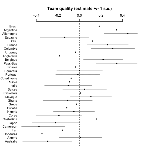
Now it's time to make some graphs. First a simple list of estimates and standard errors of team abilities. I'll order the teams based on Nate's prior ranking, which makes sense for a couple reasons. First, this ordering is informative, there's a general trend from good to bad so it should be easy to understand the results. Second, the prior ranking is what we were using to pull toward in the multilevel model, so this graph is equivalent to a plot of estimate vs. group-level predictor, which is the sort of graph I like to make to understand what the multilevel model is doing.

Here's the code:

colVars <- function(a) {n <- dim(a)[[1]]; c <- dim(a)[[2]]; return(.colMeans(((a - matrix(.colMeans(a, n, c), nrow = n, ncol = c, byrow = TRUE)) ^ 2), n, c) * n / (n - 1))}

sims <- extract(fit)
a_sims <- sims$a
a_hat <- colMeans(a_sims)
a_se <- sqrt(colVars(a_sims))
library ("arm")
png ("worldcup1.png", height=500, width=500)
coefplot (rev(a_hat), rev(a_se), CI=1, varnames=rev(teams), main="Team quality (estimate +/- 1 s.e.)\n", cex.var=.9, mar=c(0,4,5.1,2), xlim=c(-.5,.5))
dev.off()

And here's the graph:

worldcup1

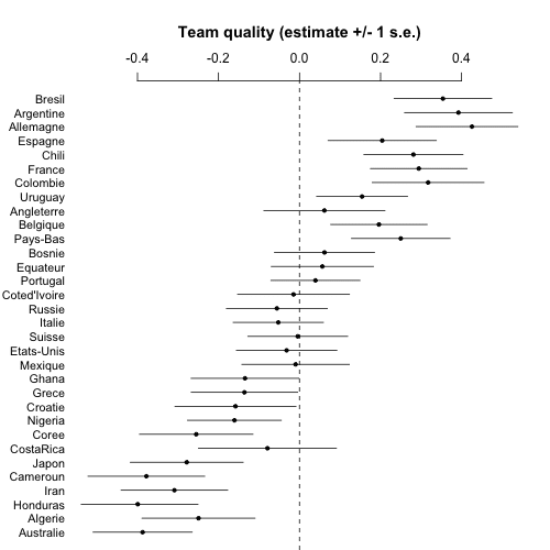
At this point we could compute lots of fun things such as the probability that Argentina will beat Germany in the final, etc., but it's clear enough from this picture that the estimate will be close to 50% so really the model isn't giving us anything for this one game. I mean, sure, I could compute such a probability and put it in the headline above, and maybe get some clicks, but what's the point?

One thing I am curious about, though, is how much of these estimates are coming from the prior ranking? So I refit the model. First I create a new Stan model, "worldcup_noprior_matt.stan", just removing the parameter "b". Then I run it from R:

fit_noprior <- stan_run("worldcup_noprior_matt.stan", data=data, chains=4, iter=100)
print(fit_noprior)

Convergence after 100 iterations is not perfect---no surprise, given that with less information available, the model fit is less stable---so I brute-force it and run 1000:

fit_noprior <- stan_run("worldcup_noprior_matt.stan", data=data, chains=4, iter=1000)
print(fit_noprior)

Now time for the plot. I could just copy the above code but this is starting to get messy so I encapsulate it into a function and run it:

worldcup_plot <- function (fit, file.png){
  sims <- extract(fit)
  a_sims <- sims$a
  a_hat <- colMeans(a_sims)
  a_se <- sqrt(colVars(a_sims))
  library ("arm")
  png (file.png, height=500, width=500)
  coefplot (rev(a_hat), rev(a_se), CI=1, varnames=rev(teams), main="Team quality (estimate +/- 1 s.e.)\n", cex.var=.9, mar=c(0,4,5.1,2), xlim=c(-.5,.5))
  dev.off()
}
worldcup_plot(fit_noprior, "worldcup1_noprior.png")

I put in the xlim values in that last line to make the graph look nice, after seeing the first version of the plot. And I also played around a bit with the margins (the argument "mar" to coefplot above) to get everything to look good. Overall, though, coefplot() worked wonderfully, straight out of the box. Thanks, Yu-Sung!

worldcup1_noprior

Similar to before but much noisier.

Act 2: Checking the fit of model to data

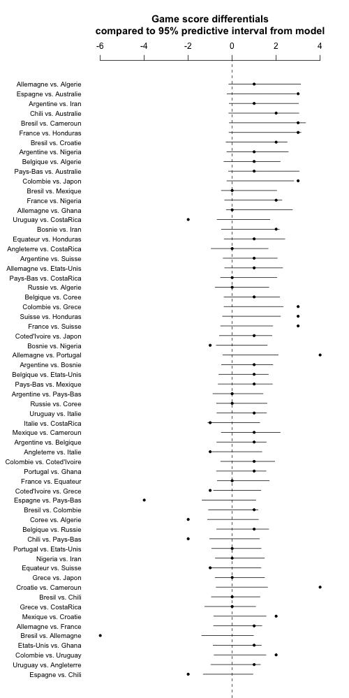
OK, fine. Now let's check model fit. For this we'll go back to the model worldcup_matt.stan which includes the prior ranking as a linear predictor. For each match we can compute an expected outcome based on the model and a 95% predictive interval based on the t distribution. This is all on the signed sqrt scale so we can do a signed square to put it on the original scale, then compare to the actual game outcomes.

Here's the R code (which, as usual, took a few iterations to debug; I'm not showing all my steps here):

expected_on_sqrt_scale <- a_hat[team1] - a_hat[team2]
sigma_y_sims <- sims$sigma_y
interval_975 <- median(qt(.975,df)*sigma_y_sims)
signed_square <- function (a) {sign(a)*a^2}
lower <- signed_square(expected_on_sqrt_scale - interval_975)
upper <- signed_square(expected_on_sqrt_scale + interval_975)

png ("worldcup2.png", height=1000, width=500)
coefplot (rev(score1 - score2), sds=rep(0, ngames),
          lower.conf.bounds=rev(lower), upper.conf.bounds=rev(upper), 
          varnames=rev(paste(teams[team1], "vs.", teams[team2])),
          main="Game score differentials\ncompared to 95% predictive interval from model\n",
          mar=c(0,7,6,2))
dev.off ()

In the code above, I gave the graph a height of 1000 to allow room for all the games, and a width of 500 to conveniently fit on the blog page. Also I went to the trouble to explicitly state in the title that the intervals were 95%.

And here's what we get:

worldcup2

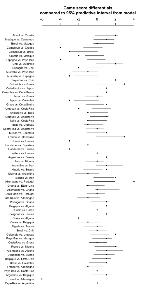
Whoa! Some majorly bad fit here. Even forgetting about Brazil vs. Germany, lots more than 5% of the points are outside the 95% intervals. My first thought was to play with the t degrees of freedom, but that can't really be the solution. And indeed switching to a t_4, or going the next step and estimating the degrees of freedom from the data (using the gamma(2,0.1) prior restricted to df>1, as recommended by Aki) didn't do much either.

Act 3: Thinking hard about the model. What to do next?

So then I got to thinking about problems with the model. Square root or no square root, the model is only approximate, indeed it's not a generative model at all, as it makes continuous predictions for discrete data. So my next step was to take the probabilities from my model, use them as predictions for each discrete score differential outcome (-6, -5, -4, . . ., up to +6) and then use these probabilities for a multinomial likelihood.

I won't copy the model in this post but it's included in the zipfile that I've attached here. The model didn't work at all and I didn't get around to fixing it.

Indeed, once we move to directly modeling the discrete data, a latent-data approach seems like it might be more reasonable, perhaps something a simple as an ordered logit or maybe something more tailored to the particular application.

Ordered logit's in the Stan manual so it shouldn't be too difficult to implement. But at this point I was going to bed and I knew I wouldn't have time to debug the model the next day (that is, today) so I resolved to just write up what I did do and be open about the difficulties.

These difficulties are not, fundamentally, R or Stan problems. Rather, they represent the challenges that arise when analyzing any new problem statistically.

Act 4: Rethinking the predictive intervals

But then, while typing up the above (it's taken me about an hour), I realized that my predictive intervals were too narrow because they're based on point estimates of the team abilities. How could I have been so foolish??

Now I'm excited. (And I'm writing here in real time, i.e. I have not yet cleaned up my code and recomputed those predictive error bounds.) Maybe everything will work out. That would make me so happy! The fractal nature of scientific revolutions, indeed.

OK, let's go to it.

*Pause while I code*

OK, that wan't too bad. First I refit the model using a zillion iterations so I can get the predictive intervals using simulation without worrying about anything:

fit <- stan_run("worldcup_matt.stan", data=data, chains=4, iter=5000)
print(fit)

Now the code:

sims <- extract (fit)
a_sims <- sims$a
sigma_y_sims <- sims$sigma_y
nsims <- length(sigma_y_sims)
random_outcome <- array(NA, c(nsims,ngames))
for (s in 1:nsims){
  random_outcome_on_sqrt_scale <- (a_sims[s,team1] - a_sims[s,team2]) + rt(ngames,df)*sigma_y_sims[s]
  random_outcome[s,] <- signed_square(random_outcome_on_sqrt_scale)
}
sim_quantiles <- array(NA,c(ngames,2))
for (i in 1:ngames){
  sim_quantiles[i,] <- quantile(random_outcome[,i], c(.025,.975))
}

png ("worldcup3.png", height=1000, width=500)
coefplot (rev(score1 - score2), sds=rep(0, ngames),
          lower.conf.bounds=rev(sim_quantiles[,1]), upper.conf.bounds=rev(sim_quantiles[,2]), 
          varnames=rev(paste(teams[team1], "vs.", teams[team2])),
          main="Game score differentials\ncompared to 95% predictive interval from model\n",
          mar=c(0,7,6,2))
dev.off ()

And now . . . the graph:

worldcup3

Hmm, the uncertainty bars are barely wider than before. So time for a brief re-think. The problem is that the predictions are continuous and the data are discrete. The easiest reasonable way to get discrete predictions from the model is to simply round to the nearest integer. So we'll do this, just changing the appropriate line in the above code to:

  sim_quantiles[i,] <- quantile(round(random_outcome[,i]), c(.025,.975))

Aaaaand, here's the new graph:

worldcup4

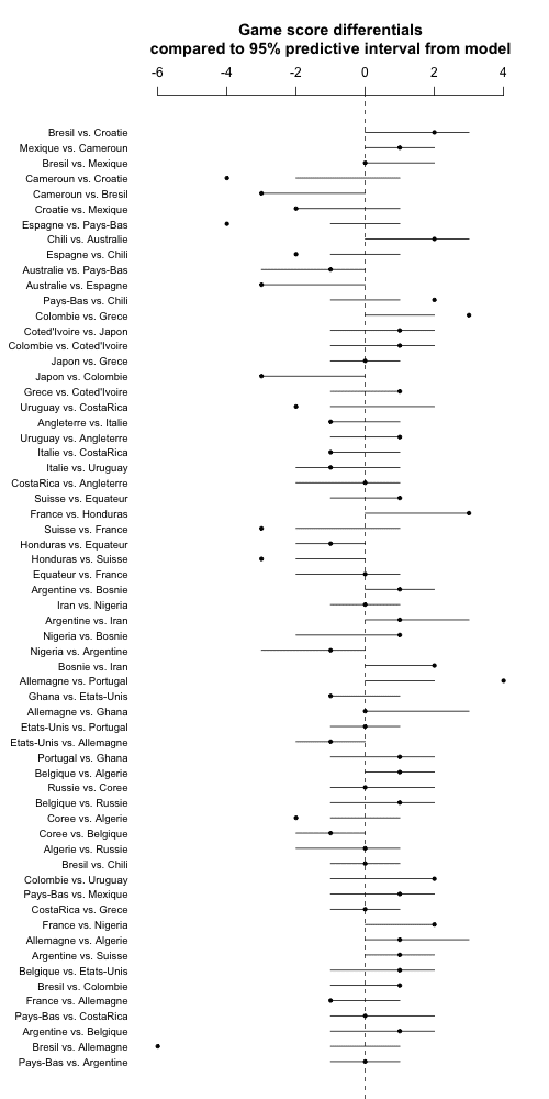
Still no good. Many more than 1/20 of the points are outside the 95% predictive intervals.

This is particularly bad given that the model was fit to the data and the above predictions are not cross-validated, hence we'd actually expect a bit of overcoverage.

One last thing: Instead of plotting the games in order of the data, I'll order them by expected score differential. I'll do it using difference in prior ranks so as not to poison the well with the estimates based on the data. Also I'll go back to the continuous predictive intervals as they show a bit more information:

a_hat <- colMeans(a_sims)
new_order <- order(a_hat[team1] - a_hat[team2])
for (i in 1:ngames){
  sim_quantiles[i,] <- quantile(random_outcome[,i], c(.025,.975))
}
png ("worldcup5.png", height=1000, width=500)
coefplot ((score1 - score2)[new_order], sds=rep(0, ngames),
          lower.conf.bounds=sim_quantiles[new_order,1], upper.conf.bounds=sim_quantiles[new_order,2], 
          varnames=paste(teams[team1[new_order]], "vs.", teams[team2[new_order]]),
          main="Game score differentials\ncompared to 95% predictive interval from model\n",
          mar=c(0,7,6,2))
dev.off ()

worldcup5

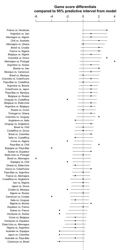
Hey, this worked on the first try! Cool.

But now I'm realizing one more thing. Each game has an official home and away team but this direction is pretty much arbitrary. So I'm going to flip each game so it's favorite vs. underdog, with favorite and underdog determined by the prior ranking.

So here it is, with results listed in order from expected blowouts to expected close matches:

worldcup6

Again, lots of outliers, indicating that my model sucks. Maybe there's also some weird thing going on with Jacobians when I'm doing the square root transformations. Really I think the thing to do is to build a discrete-data model. In 2018, perhaps.

Again, all the data and code are here. (I did not include last night's Holland/Brazil game but of course it would be trivial to update the analyses if you want.)

P.S. In the 9 June post linked above, Nate wrote that his method estimates that "a 20 percent chance that both the Netherlands and Chile play up to the higher end of the range, or they get a lucky bounce, or Australia pulls off a miracle, and Spain fails to advance despite wholly deserving to." I can't fault the estimate---after all, 1-in-5 events happen all the time---but I can't see why he was so sure that if Spain loses, that they still wholly deserved to win. They lost 5-1 to Holland and 2-0 to Chile so it doesn't seem like just a lucky bounce. At some point you have to say that if you lost, you got what you deserved, no?

P.P.S. The text in those png graphs is pretty hard to read. Would jpg be better? I'd rather not use pdf because then I'd need to convert it into an image file before uploading it onto the blog post.

P.P.P.S. I found a bug! The story is here.

(Py, R, Cmd) Stan 2.3 Released

We’re happy to announce RStan, PyStan and CmdStan 2.3.
Instructions on how to install at:

As always, let us know if you’re having problems or have comments or suggestions.

We’re hoping to roll out the next release a bit quicker this time, because we have lots of good new features that are almost ready to go (vectorizing multivariate normal, higher-order autodiff for probability functions, differential equation solver, L-BFGS optimizer).

Here are the official release notes.

v.2.3.0 (18 June 2014)
======================================================================

We had a record number of user-submitted patches this go around.
Thanks to everyone!

New Features
------------
* user-defined function definitions added to Stan language
* cholesky_corr data type for Cholesky factors of correlation matrices
* a^b syntax for pow(a,b)  (thanks to Mitzi Morris)
* reshaping functions: to_matrix(), to_vector(), to_row_vector(), 
  to_array_1d(), to_array_2d()
* matrix operations: quad_form_sym() (x' *Sigma * x), QR decompositions
  qr_Q(), qr_R()
* densities: Gaussian processes multi_gp_log(), multi_gp(), 
  and alternative negative binomial parameterization neg_binomial_2()
* random number generator: multi_normal_cholesky_rng()
* sorting: sort_indices_*() for returning indexes in sorted order by
  value
* added JSON parser to C++ (not exposed through interfaces yet; thanks
  to Mitzi Morris)
* many fixes to I/O for data and inits to check consistency and
  report errors
* removed some uses of std::cout where they don't belong
* updated parser for C++11 compatibility (thanks to Rob Goedman)

New Developer
--------------
* added Marco Inacio as core developer

Optimizations
-------------
* turned off Eigen asserts
* efficiency improvements to posterior analysis print

Documentation
-------------
* Clarified licensing policy for individual code contributions
* Huge numbers of fixes to the documentation, including many
  user-contributed patches (thanks!), fixes to parallelization in
  CmdStan, Windows install instructions, boundaries for Dirichlet and
  Beta, removed suggestion to use floor and ceiling as indices,
  vectorized many models, clarified that && doesn't short circuit,
  clarified von Mises normalization, updated censoring doc (thanks
  to Alexey Stukalov), negative binomial doc enhanced, new references,
  new discussion of hierarchical models referencing Betancourt and
  Girolami paper, 
* Avraham Adler was particularly useful in pointing out and fixing
  documentation errors

Bug Fixes
------------
* fixed bug in lkj density
* fixed bug in Jacobian for corr_matrix data type
* fix cholesky_cov_matrix test code to allow use as parameter
* fixed poisson_rng, neg_binomial_rng
* allow binary operations (e.g., < and >) within range constraints
* support MS Visual Studio 2008
* fixed memory leaks in categorical sampling statement, categorical_log
  function, and softmax functions
* removed many compiler warnings
* numerous bug fixes to arithmetic test code conditions and messages,
  including calls from 
* fixed model crashes when no parameter specified
* fixed template name conflicts for some compiler bugs (thanks Kevin
  S. Van Horn)

Code Reorganizations & Updates
------------------------------
* CmdStan is now in its own repository on GitHub: stan-dev/cmdstan
* consolidate and simplify error handling across modules
* pulled functionality from CmdStan command class and PyStan and RStan
  into Stan C++
* generalized some interfaces to allow std::vector as well as Eigen
  for compatibility
* generalize some I/O CSV writer capabilities
* optimization output text cleaned up
* integer overflow during I/O now raises informative error messages
* const correctness for chains (thanks Kevin S. Van Horn)

Identifying pathways for managing multiple disturbances to limit plant invasions

Andrew Tanentzap, William Lee, Adrian Monks, Kate Ladley, Peter Johnson, Geoffrey Rogers, Joy Comrie, Dean Clarke, and Ella Hayman write:

We tested a multivariate hypothesis about the causal mechanisms underlying plant invasions in an ephemeral wetland in South Island, New Zealand to inform management of this biodiverse but globally imperilled habitat. . . . We found that invasion by non-native plants was lowest in sites where the physical disturbance caused by flooding was both intense and frequent. . . . only species adapted to the dominant disturbance regimes at a site may become successful invaders.

Their keywords are:

causal networks; community dynamics; functional traits, invasive species, kettlehole; megafauna; rabbits; restoration; turf plants

But here’s the part that I like best:

We fitted all our models within a hierarchical Bayesian framework using . . . STAN v.1.3 (Stan Development Team 2012) from R v.2.15 (R Development Core Team 2012).

Bayesian nonparametric weighted sampling inference

Yajuan Si, Natesh Pillai, and I write:

It has historically been a challenge to perform Bayesian inference in a design-based survey context. The present paper develops a Bayesian model for sampling inference using inverse-probability weights. We use a hierarchical approach in which we model the distribution of the weights of the nonsampled units in the population and simultaneously include them as predictors in a nonparametric Gaussian process regression. We use simulation studies to evaluate the performance of our procedure and compare it to the classical design-based estimator. We apply our method to the Fragile Family Child Wellbeing Study. Our studies find the Bayesian nonparametric finite population estimator to be more robust than the classical design-based estimator without loss in efficiency.

Screen Shot 2014-05-28 at 8.57.01 AM

More work needs to be done for this to be a general practical tool—in particular, in the setup of this paper you only have survey weights and no direct poststratification variables—but at the theoretical level I think it’s a useful start, because it demonstrates how we can feed survey weights into a general Mister P framework in which the poststratification population sizes are unknown and need to be estimated from data. I’m very excited about this general line of research. (And we’re fitting the model in Stan.)

Transitioning to Stan

Kevin Cartier writes:

I’ve been happily using R for a number of years now and recently came across Stan. Looks big and powerful, so I’d like to pick an appropriate project and try it out. I wondered if you could point me to a link or document that goes into the motivation for this tool (aside from the Stan user doc)? What I’d like to understand is, at what point might you look at an emergent R project and advise, “You know, that thing you’re trying to do would be a whole lot easier/simpler/more straightforward to implement with Stan.” (or words to that effect).

My reply: For my collaborators in political science, Stan has been most useful for models where the data set is not huge (e.g., we might have 10,000 data points or 50,000 data points but not 10 million) but where the model is somewhat complex (for example, a model with latent time series structure). The point is that the model has enough parameters and uncertainty that you’ll want to do full Bayes (rather than some sort of point estimate). At that point, Stan is a winner compared to programming one’s own Monte Carlo algorithm.

We (the Stan team) should really prepare a document with a bunch of examples where Stan is a win, in one way or another. But of course preparing such a document takes work, which we’d rather spend on improving Stan (or on blogging…)

Stan Model of the Week: PK Calculation of IV and Oral Dosing

[Update: Revised given comments from Wingfeet, Andrew and germo. Thanks! I’d mistakenly translated the dlnorm priors in the first version — amazing what a difference the priors make. I also escaped the less-than and greater-than signs in the constraints in the model so they’re visible. I also updated to match the thin=2 output of JAGS.]

We’re going to be starting a Stan “model of the P” (for some time period P) column, so I thought I’d kick things off with one of my own. I’ve been following the Wingvoet blog, the author of which is identified only by the Blogger handle Wingfeet; a couple of days ago this lovely post came out:

Wingfeet’s post implemented an answer to question 6 from chapter 6 of problem from Rowland and Tozer’s 2010 book, Clinical Pharmacokinetics and Pharmacodynamics, Fourth edition, Lippincott, Williams & Wilkins.

So in the grand tradition of using this blog to procrastinate, I thought I’d take a break from C++ coding and paper writing and translate Wingfeet’s model to Stan. First, let me repeat Wingfeet’s model in JAGS, exactly as posted:

  tau <- 1/pow(sigma,2)
  sigma ~ dunif(0,100)
# IV part
  kIV ~dnorm(.4,1)
  cIV ~ dlnorm(1,.01)
  for (i in 1:nIV) {
    predIV[i] <- c0*exp(-k*timeIV[i]) +cIV*exp(-kIV*timeIV[i])
    concIV[i] ~ dnorm(predIV[i],tau)
  }
  c0 <- doseIV/V
  V ~ dlnorm(2,.01)
  k <- CL/V
  CL ~ dlnorm(1,.01)
  AUCIV <- doseIV/CL+cIV/kIV
# oral part
  for (i in 1:nO) {
    predO[i] <- c0star*(exp(-k*timeO[i])-exp(-ka*timeO[i]))
    concO[i] ~ dnorm(predO[i],tau)
  }
  c0star <- doseO*(ka/(ka-k))*F/V
  AUCO <- c0star/k
  F ~ dunif(0,1)
  ka ~dnorm(.4,1)
  ta0_5 <- log(2) /ka
  t0_5 <- log(2)/k

I still find JAGS models pretty hard to follow on their own, but Wingfeet provided the data, and the call to R2Jags, so I could work backwards from there. Here's what I came up with as a translation to Stan.

data {
  int<lower=0> nIV;
  int<lower=0> nOral;
  real<lower=0> doseIV;
  real<lower=0> doseOral;
  vector<lower=0>[nIV] timeIV;
  vector<lower=0>[nIV] concIV;
  vector<lower=0>[nOral] timeOral;
  vector<lower=0>[nOral] concOral;
}
parameters {
  real<lower=0> CL;
  real<lower=0> V;
  real<lower=0,upper=1> F;
  real<lower=0> ka; 
  real<lower=0> kIV; 
  real<lower=0> cIV; 
  real<lower=0,upper=100> sigma;
}
transformed parameters {
  real k;
  real c0;
  real AUCIV;
  real c0star;
  real AUCOral;
  real ta0_5;
  real t0_5;
  vector[nIV] predIV;
  vector[nOral] predOral;

  k <- CL / V;
  c0 <- doseIV / V;
  AUCIV <- doseIV / CL + cIV / kIV;
  c0star <- doseOral * (ka / (ka - k)) * F / V;
  AUCOral <- c0star / k;
  ta0_5 <- log(2) / ka;
  t0_5 <- log(2) / k;
  predIV <- c0 * exp(-k * timeIV) + cIV * exp(-kIV * timeIV);
  predOral <- c0star * (exp(-k * timeOral) - exp(-ka * timeOral));
}
model {
  // IV component
  kIV ~ normal(0.4, 1);
  cIV ~ lognormal(1,10);
  V ~ lognormal(2,10);
  CL ~ lognormal(1,10);
  concIV ~ normal(predIV, sigma);

  // oral component
  ka ~ normal(0.4,1);
  concOral ~ normal(predOral, sigma);
}

Do I ever appreciate the emacs mode for Stan! The Stan model is a direct translation of Wingfeet's JAGS model, with exactly the same priors (Stan uses a sd parameterization of the normal, whereas JAGS follows bugs in using inverse variance). I moved all the deterministic nodes in the JAGS model to the transformed parameters block in the Stan model so we could inspect them in the output. I also vectorized the prediction calculations, which seems much cleaner than using loops, but opinions may vary on this point.

It was critical to put the lower-bounds on all the concentration and volume parameters in Stan, as well as upper and lower bounds on the noise term (which had a broad uniform distribution in the JAGS model).

Here's the data in Stan's dump format, which I dropped in a file named data.R:

nIV <- 12
nOral <- 11
doseIV <- 500
doseOral <- 500
timeIV <- 
c(0.33, 0.5, 0.67, 1.5, 2, 4, 6, 10, 16, 24, 32, 48)
concIV <- 
c(14.7, 12.6, 11, 9, 8.2, 7.9, 6.6, 6.2, 4.6, 3.2, 2.3, 1.2)
timeOral <- 
c(0.5, 1, 1.5, 2, 4, 6, 10, 16, 24, 32, 48)
concOral <- 
c(2.4, 3.8, 4.2, 4.6, 8.1, 5.8, 5.1, 4.1, 3, 2.3, 1.3)

Here's the code to run it in RStan, with number of warmup iterations and sampling iterations matching Wingfeet's call to the R2Jags package.

library('rstan');
source('data.R');
fit <- stan('pk_iv_oral.stan', 
            data=c("nIV","nOral","doseIV","doseOral", 
                   "timeIV","concIV","timeOral","concOral"),
            chains=4, warmup=5000, iter=14000);

It took about 10s to compile the model and 8s to run 56K iterations in the release version of RStan 2.2.0 (on my several years old Macbook Pro with 2.3GHz Intel Core i7). This uses the default diffuse initializations drawn uniformly on (-2,2) on the unconstrained scale corresponding to roughly (0.1, 10) on the positive-constrained scale

The model converged almost instantly and mixes very well, so this number of iterations is rather an overkill for Stan. Note that I set Stan to thin every other draw, to match the JAGS configuration used by Wingfeet.

nference for Stan model: pk_iv_oral.
4 chains, each with iter=14000; warmup=5000; thin=2; 
post-warmup draws per chain=4500, total post-warmup draws=18000.

               mean se_mean    sd   2.5%    25%    50%    75%  97.5% n_eff Rhat
CL             2.35    0.00  0.18   2.00   2.23   2.34   2.46   2.72 13417    1
V             56.44    0.02  2.70  51.73  54.62  56.25  58.00  62.39 12204    1
F              0.87    0.00  0.05   0.77   0.84   0.87   0.91   0.97 12223    1
ka             0.66    0.00  0.10   0.49   0.59   0.65   0.72   0.90 12383    1
kIV            2.08    0.00  0.51   1.16   1.72   2.05   2.41   3.14 11219    1
cIV           11.30    0.02  2.47   7.20   9.57  11.05  12.73  16.90 11978    1
sigma          0.57    0.00  0.11   0.41   0.50   0.56   0.64   0.84 10536    1
k              0.04    0.00  0.00   0.03   0.04   0.04   0.04   0.05 12654    1
c0             8.88    0.00  0.42   8.01   8.62   8.89   9.15   9.67 12448    1
AUCIV        219.90    0.15 16.88 189.43 208.69 219.01 230.17 256.13 13048    1
c0star         8.31    0.01  0.61   7.15   7.91   8.29   8.69   9.56 12398    1
AUCOral      200.25    0.12 14.91 172.41 190.34 199.78 209.56 230.64 14644    1
ta0_5          1.08    0.00  0.16   0.77   0.97   1.07   1.18   1.42 12769    1
t0_5          16.79    0.02  1.69  13.82  15.67  16.64  17.75  20.57 12133    1
predIV[1]     14.36    0.00  0.52  13.29  14.02  14.37  14.70  15.35 13530    1
predIV[2]     12.64    0.00  0.33  11.99  12.43  12.63  12.85  13.29 17290    1
predIV[3]     11.43    0.00  0.35  10.75  11.19  11.42  11.66  12.13 14406    1
predIV[4]      8.92    0.00  0.32   8.33   8.70   8.90   9.11   9.60 14157    1
predIV[5]      8.41    0.00  0.29   7.85   8.22   8.40   8.59   9.00 14461    1
predIV[6]      7.52    0.00  0.28   6.94   7.34   7.53   7.71   8.06 13229    1
predIV[7]      6.91    0.00  0.25   6.39   6.75   6.92   7.08   7.39 13267    1
predIV[8]      5.85    0.00  0.22   5.40   5.71   5.85   6.00   6.28 13885    1
predIV[9]      4.56    0.00  0.23   4.10   4.41   4.56   4.71   5.01 13958    1
predIV[10]     3.27    0.00  0.25   2.78   3.11   3.27   3.43   3.77 13481    1
predIV[11]     2.35    0.00  0.25   1.87   2.19   2.34   2.51   2.86 13122    1
predIV[12]     1.22    0.00  0.21   0.84   1.08   1.20   1.34   1.66 12692    1
predOral[1]    2.14    0.00  0.21   1.74   2.00   2.13   2.27   2.59 14328    1
predOral[2]    3.63    0.00  0.29   3.06   3.43   3.62   3.81   4.23 14973    1
predOral[3]    4.65    0.00  0.30   4.05   4.46   4.65   4.85   5.26 15721    1
predOral[4]    5.35    0.00  0.29   4.76   5.16   5.36   5.54   5.91 16427    1
predOral[5]    6.37    0.00  0.27   5.81   6.20   6.38   6.56   6.89 15049    1
predOral[6]    6.27    0.00  0.30   5.64   6.08   6.28   6.48   6.84 13781    1
predOral[7]    5.45    0.00  0.29   4.87   5.27   5.45   5.64   6.01 13940    1
predOral[8]    4.26    0.00  0.24   3.78   4.10   4.26   4.42   4.73 14936    1
predOral[9]    3.05    0.00  0.22   2.62   2.91   3.05   3.20   3.49 14965    1
predOral[10]   2.19    0.00  0.22   1.78   2.05   2.19   2.33   2.63 14373    1
predOral[11]   1.13    0.00  0.18   0.81   1.01   1.12   1.24   1.51 13457    1
lp__          -2.09    0.03  2.33  -7.80  -3.33  -1.68  -0.37   1.19  7734    1

Samples were drawn using NUTS(diag_e) at Tue Mar 11 01:48:42 2014.

Here's the fit that Wingfeet got from JAGS:

Inference for Bugs model at "C:/...BEnL/model1b6027171a7a.txt", fit using jags,
 4 chains, each with 14000 iterations (first 5000 discarded), n.thin = 2
 n.sims = 18000 iterations saved
           mu.vect sd.vect    2.5%     25%     50%     75%   97.5%  Rhat n.eff
AUCIV      219.959  16.975 189.743 208.636 218.846 230.210 256.836 1.002  2800
AUCO       200.468  15.102 171.908 190.523 199.987 209.928 231.722 1.001  7500
CL           2.346   0.182   1.995   2.226   2.344   2.461   2.712 1.002  2900
F            0.876   0.052   0.773   0.841   0.876   0.911   0.976 1.002  3200
V           56.463   2.752  51.610  54.583  56.280  58.112  62.465 1.002  3100
c0           8.876   0.426   8.005   8.604   8.884   9.160   9.688 1.002  3100
c0star       8.314   0.615   7.119   7.911   8.304   8.704   9.574 1.002  2000
cIV         11.229   2.485   7.029   9.511  11.003  12.654  16.804 1.003  1100
k            0.042   0.004   0.034   0.039   0.042   0.044   0.050 1.002  2200
kIV          2.064   0.510   1.132   1.704   2.041   2.396   3.126 1.004   800
ka           0.659   0.105   0.489   0.589   0.646   0.715   0.903 1.002  3200
predIV[1]   14.343   0.532  13.240  14.009  14.355  14.690  15.378 1.002  2500
predIV[2]   12.637   0.331  11.990  12.422  12.632  12.851  13.298 1.001 12000
predIV[3]   11.435   0.357  10.755  11.196  11.427  11.667  12.147 1.002  1600
predIV[4]    8.923   0.326   8.333   8.709   8.902   9.116   9.638 1.002  2900
predIV[5]    8.410   0.298   7.845   8.213   8.401   8.594   9.021 1.001 14000
predIV[6]    7.522   0.286   6.943   7.340   7.525   7.713   8.064 1.001  5900
predIV[7]    6.910   0.255   6.385   6.749   6.915   7.077   7.399 1.001  6200
predIV[8]    5.848   0.222   5.406   5.704   5.849   5.993   6.285 1.001  7800
predIV[9]    4.557   0.231   4.098   4.409   4.555   4.707   5.012 1.001  4500
predIV[10]   3.270   0.252   2.781   3.107   3.267   3.433   3.773 1.002  3100
predIV[11]   2.349   0.251   1.867   2.183   2.343   2.509   2.865 1.002  2700
predIV[12]   1.217   0.207   0.839   1.076   1.204   1.343   1.662 1.002  2500
predO[1]     2.138   0.214   1.750   1.995   2.124   2.263   2.599 1.001  8700
predO[2]     3.626   0.293   3.070   3.432   3.616   3.807   4.234 1.001 12000
predO[3]     4.653   0.306   4.050   4.452   4.652   4.847   5.264 1.001 16000
predO[4]     5.351   0.294   4.754   5.161   5.354   5.541   5.930 1.001 15000
predO[5]     6.375   0.277   5.801   6.202   6.383   6.562   6.894 1.002  3200
predO[6]     6.274   0.308   5.629   6.079   6.286   6.485   6.842 1.002  2800
predO[7]     5.455   0.292   4.852   5.270   5.461   5.648   6.018 1.002  3900
predO[8]     4.262   0.245   3.764   4.106   4.265   4.423   4.736 1.001  8600
predO[9]     3.057   0.227   2.605   2.910   3.058   3.207   3.504 1.001  8200
predO[10]    2.195   0.218   1.773   2.050   2.192   2.335   2.638 1.001  5200
predO[11]    1.135   0.180   0.805   1.013   1.127   1.247   1.519 1.002  3500
t0_5        16.798   1.713  13.830  15.655  16.652  17.770  20.617 1.002  2200
ta0_5        1.077   0.164   0.768   0.969   1.072   1.177   1.419 1.002  3200
deviance    38.082   5.042  30.832  34.357  37.207  40.918  50.060 1.003  1200

Stan mixed better, but I should add that with thin=1, the number effective samples increased dramatically --- Stan's making nearly independent draws each iteration. Wingfeet reports that the "correct" answers (presumably given in the book) were the following, here reported with the 95% posterior intervals produced by Stan and JAGs (we've been meaning to reduce RStan's posterior intervals to 90% to match CmdStan's, but it hasn't happened yet):

 
Parameter   Correct          Stan 95%       JAGS 95%
---------   -----------    ------------    ------------
t0_5        16.7 hr        (13.8,  20.6)    (13.8, 20.6)
AUCiv       217 mg-hr/L    ( 189,   256)    ( 190,  256)      
AUCoral     191 mg-hr/L    ( 172,   231)    ( 172,  232)
CL          2.3 L/hr       ( 2.0,   2.7)    ( 2.0,  2.7)
V           55 L           (51.7,  62.4)    (51.6, 62.5)
F           0.88           (0.77,  0.97)    (0.77, 0.98)

It's nice to see two completely different approaches (HMC and generalized Gibbs/slice) give the same answers.