Subtle statistical issues to be debated on TV.

There is live debate that will available this week for those that might be interested. The topic: Can early stopped trials result in misleading results of systematic reviews?

It’s sponsored by the Cochrane Collaboration and although the level of discussion is often not very technical, it does in my opinion provide a nice window into clinical research and as Tukey might put it “the real uncertainties involved”.

(As a disclaimer – I once assigned some reading from this group to my graduate students and they were embarrassed and annoyed at the awkward handling of even minor technical issues – but the statistical research community is not their target audience.)

I have a favourite in this debate, and a quick search on co-authors (not me) would likely tip that off to most members of this blog.

Here’s the directions kindly supplied by Jonathan Sterne, who will be in the chair.

Dear SMG Members,

By means of follow up to previous advertisements; the Discussion Meeting:”Can early stopped trials result in misleading results of systematic reviews?” will be broadcast live online (please see attached for further meeting details).

October 21 2010, 07.30 – 09.00 AM Denver Time (MDT)
(US East Coast +2 hours, UK +7, Central European Time plus 8)

To watch the meeting live, simply visit: www.cochrane.tv at your equivalent local time.

Should you have any queries or comments, before or after the meeting please do not hesitate to get in touch.

Jonathan Sterne

———————-

Jonathan Sterne
School of Social and Community Medicine
University of Bristol

Abstract

Can early stopped trials result in misleading results
of systematic reviews?
Cochrane Colloquium, Keystone Colorado
October 21 2010, 07.30-09.00

Following the publication of empirical studies demonstrating differences between the results of trials that are stopped early and those that continue to their planned end of follow up, there has been intensive recent debate about whether the results of stopped early trials can mislead the clinician and consumer public. The Cochrane Bias Methods Group and Statistical Methods Group are delighted that two leading experts have agreed to present their views and lead a discussion on how review authors should address this issue.

Stopping early for benefit: is there a problem, and if so, what is it? Gordon Guyatt, McMaster University

Stopping at nothing? Some Dilemmas of Data Monitoring in Clinical Trials
Steven Goodman, Johns Hopkins University Schools of Medicine and Public Health

K?

Course proposal: Bayesian and advanced likelihood statistical methods for zombies.

The course outline

ZombieCourseOutline.rtf

Hints/draft R code for implementing this for a regression example from D. Pena
x=c(1:10,17,17,17)
y=c(1:10,25,25,25)

ZombieAssign1.txt

The assignment being to provide a legend that explains all the lines and symbols in this plot

ZombieAssign1.pdf

With a bonus assignment being to provide better R code and or techniques.

And a possible graduate student assignment to investigate what percentage of examples in graduate stats texts (e.g. Cox & Hinkley) could be displayed this way (reducing the number of parameters to least number possible).

K?
p.s. might have been a better post for Friday the 13th
p.s.2 background material from my thesis (passed in 2007)
ThesisReprint.pdf

UnConMax – uncertainty consideration maxims 7 +/- 2

Warning – this blog post is meant to encourage some loose, fuzzy and possibly distracting thoughts about the practice of statistics in research endeavours. There maybe spelling and grammatical errors as well as a lack of proper sentence structure. It may not be understandable to many or even possibly any readers.

But somewhat more seriously, its better that “ConUnMax”

So far I have five maxims

1. Explicit models of uncertanty are useful but – always wrong and can always be made less wrong
2. If the model is formally a probability model – always use probability calculus (Bayes)
3. Always useful to make the model a formal probability model – no matter what (Bayesianisn)
4. Never use a model that is not empirically motivated and strongly empirically testable (Frequentist – of the anti-Bayesian flavour)
5. Quantitative tools are always just a means to grasp and manipulate models – never an end in itself (i.e. don’t obsess over “baby” mathematics)
6. If one really understood statistics, they could always successfully explain it to any zoombie

K?

Should Mister P be allowed/encouraged to reside in counter-factual populations?

Lets say you are repeatedly going to recieve unselected sets of well done RCTs on various say medical treatments.

One reasonable assumption with all of these treatments is that they are monotonic – either helpful or harmful for all. The treatment effect will (as always) vary for subgroups in the population – these will not be explicitly identified in the studies – but each study very likely will enroll different percentages of the variuos patient subgroups. Being all randomized studies these subgroups will be balanced in the treatment versus control arms – but each study will (as always) be estimating a different – but exchangeable – treatment effect (Exhangeable due to the ignorance about the subgroup memberships of the enrolled patients.)

That reasonable assumption – monotonicity – will be to some extent (as always) wrong, but given that it is a risk believed well worth taking – if the average effect in any population is positive (versus negative) the average effect in any other population will be positive (versus negative).

If we define a counter-factual population based on a mixture of the study’s unknown mixtures of subgroups – by inverse variance weighting of the study’s effect estimates by their standard errors – we would get an estimate of the average effect for that counter-factual population that is minimum variance (and the assumptions rule out much – if any bias in this).

Should we encourage (or discourage) such Mr P based estimates – just because they are for counter-factual rather than real populations.

K?

Zombie student manipulation of symbols/taking of course notes

As with those who manipulate symbols without reflective thought, that Andrew raised, I was recently thinking abouts students who avoid any distraction that might arise by their thinking about what the lecturer is talking about – so that they are sure to get the notes just right.

When I was a student I would sometimes make a deal where someone else would take the notes and I would just listen – then I would correct the notes they took for misconceptions later – there were almost always quite a few.

But not to be disparaging of students – they learned this somewhere/how and there must be advantages.

In fact – in someways math is a discouragement of thinking – replacing thinking with symbol manipulation thats assured to avoid wrong answers … to the now zombified assumptions.

K?

When engineers fail the bridge falls down: When statisticians fail millions of dollars of scarce research funding is squandered and serious public health issues are left far more uncertain than they needed to be

Saw a video link talk at a local hospital based research institute last Friday

Usual stuff about a randomized trail not being properly designed nor analyzed – as if we have not heard about that before

But this time is was tens of millions of dollars and a health concern that likely directly affects over 10% of the readers of this blog – the males over 40 or 50 and those that might care about them

Its was a very large PSA screening study and and

the design and analysis apparently failed to consider the _usual_ and expected lag in a screening effect here (perhaps worth counting the number of statisticians in the supplementary material given)

for an concrete example from colon cancer see here

And apparently a proper reanalysis was initially hampered by the well known – “we would like to give you the data but you know” …. but eventually a reanalysis was able to recover enough of the data from the from published documents

but even with the proper analysis – the public health issue – does PSA screening do more good than harm ( half of US currently males get PSA screening at some time? ) will likely remain largely uncertain or at least more uncertain than it needed to be

and it will happen again and again (seriously wasteful and harmful design and analysis)

and there will be a lot more needless deaths from either “screening being adopted” if it truly shouldn’t have been or “screening was not more fully adopted, earlier” when it truly should have been (there can be very nasty downsides from ineffective screening programs, including increased mortality)

OK I remember being involved in this PSA screening stuff many years ago in Toronto and think we argued that given the size of the study required – scarce research dollars would likely have a much better return studying some other health concerns (most of us were males but young)

But the PSA screening studies were funded – but apparently defectively designed and analyzed.

Now I had been involved in the design of a liver screening trial around 1990 (not funded because it was percieved as being too expensive) and the lag of an effect did not actually occur to me

until I started to write up the power simulation studies (discouraged by my advisor who told me professional statisticians should not have to stoop to simulations to calculate power)

and then I had to think up a treatment effect.

The immediate effect would likely not appear right away – the early treatable tumours would not have a mortality outcome for a while – after all they were early.

But maybe as important – I did some literature searching (breaking Ripley’s rule that statisticians don’t read the literature) and there were papers discussing the lag effect in treatment effects in screening trials and they suggested ways to design and analyze given these.

Then to hear of a huge disaster happening much later – in the 2000,s – why does it happen?

Statisticians have to think through the biological details of studies – somehow

Simulating planned trials is very important – even if you can get away with (i.e. fool reviewers) highly non-robust over simplified closed form professional looking power formulas

Statisticians have to confer widely – especially when designing a large expensive trial

Anyone can be “blind sided”

Do literature searches specifically on the study design and clinical topic

Read some of that literature

Try to contact other statisticians who have worked with such designs and that clinical topic

Try to have some of them look at your design

Simulate the details – that’s were the devils are

And if you notice someone else has blown it and you could fix it if you just could get their data…

Well you should be able to get their data – but there are good and not so good reasons why that won’t be feasible – but sometimes you can get more from the published data that you might think

First and technically challenging – there is always the marginal likelihood – the probablity of the published (rather than actual|) observations gives the appropriate likelihood (some math details here “justimportance.pdf” )

But sometimes you can get everything:

under Normal assumptions just the means and variances are sufficient (that just means the marginal likelihood exactly equals the full data likelihood)

in correspondence analysis there is something called the Burt matrix which is a summary from which you can (with some algebra) redo the full correspondence analysis as if you had the actual data

and for survival data the Kaplan-Meier curve – with enough resolution – will allow you to read off the raw data (event and censoring times). Modern pdf’s can provide full resolution?

Perhaps most importantly to avoid statistical bridges falling down:

We should try to worry more about public health rather our public (professional) images or even our publications!

K?

Statistics is easy! part 2.F making it look easy was easy with subtraction rather than addition

After pointing out that getting a true picture of how log prior and log likelihood add to get the log posterior – was equivalent to getting a fail safe diagnostic for MCMC convergence

I started to think that was bit hard – to just get a display to show stats was easy …

But then why not just subtract?

From the WinBugs MCMC output just get a density estimate of the log posterior and subtract the log prior to get the log likelihood to plot.

Ok its no longer a diagnostic and I’ll need to read up on how to do the density estimation better – but these wiggly lines added to the plot below completes the project

plot4.png

Keeping the log likelihood from the error prone numerical integration and the green one from the sometimes _wonky_ profiling on the plot does serve as fallible MCMC convergence diagnostics.

Now I really do believe plots like these should used in practice – especially by new novice Bayesians and recent grads – but how to help make that happen?

As a reviewer once said of something related (about 20 years ago) “it would not be of interest to a professional statistical audience” – but perhaps blogging about it is a good first step.

And I should use the multiple runs idea as in this plot
plot5.png

K?

Statistics is easy! part 2.1 – can we avoid unexpected bumps when making it look easy?

I increased the range of the plot from Statistics is easy! part 2 and added the 2.5% and 97.5% percentiles from a WinBugs run on the same problem … using bugs() of course

And then started to worry about that nasty bump on the right of the 97.5% percentiles

plot3.png

Did not take long to realize the default numerical integration was failing – too bad it did so – so smoothly.

Located a program I wrote a couple years ago to do _guaranteed_ upper and lower bounds for integrals based on envelope rules by Evans and Swartz – too bad I did not write comments in it.

But I did confirm the above is very close at log odds of 2 and definitely too high at log odds of 6. With some more careful programing I soon should be able to get upper and lower curves that bound where the integrated log likelihood should be!

But it does seem like a lot of work to make such a simple problem look easy.

But then, it would by a _fail safe_ diagnostic for MCMC convergence

for problems involving just 2 parameters
( and the guarantee and fail safe do depend on some contions )

Maybe statistics was not meant to be made to look easy.

K?

Statistics is easy! part 2 – can we at least make it look easy?

Well can we at least make it look easy?

For the model as given here, there are two parameters Pc and Pt – but the focus of interest will be on some parameter representing a treatment effect
– Andrew chose Pt – Pc.

But sticking for a while with Pt and Pc – the prior is a surface over Pt and Pc as is the data model (likelihood)

In particular, the prior is a flat surface (independent uniforms)
and the likelihood is Pt^1 (1 – Pt)^29 * Pc^3 (1 – Pc)^7 (the * is from independence)

(If I reversed the treatment and control groups – I should be blinded to that anyways)

Since the posterior is proportional to prior * likelihood we take logs and suggest plotting 3 surfaces LogPrior, Loglikelihood, and LogPosterior (i.e. LogPrior + LogLikelihood)
– along with a tracing out of a region of highest posterior probability or some simple approximation of that.

This shows all inference pieces and their sum (summative inference) in this problem.
If researchers could think in clearly in two dimensions we would be done.

Regardless the convention is to think in one dimension so …

Transform Pt and Pc into (Pt-Pc) and Pc; and then focus on just (Pt-Pc)
– now just a curve.

This is (formally) easy to do with the posterior (integrate out Pc from the surface to get a curve for just (Pt-Pc)).

Andrew’s simple method, I believe depends on (knowing) the quadratic curve centered at (Pt-Pc) with curvature = -1/(Pt * (1-Pt)/nt + Pc * (1-Pc)/nc) in the (Pt-Pc) axis but constant in the Pc axis
– approximates the poserior surface well as does going down two units from the maximum to get an interval.

Maybe not all statisticians will immediately get this – on first look.

But it would be nice to still show the pieces and how they add in one dimension.

Fortunately in most Bayesian analyses, this is (formally) possible with no loss (see this paper)

– any posterior curve for a parameter of focus (obtained by integrating out the other parameters from the surface) can be rewritten as

Integrated posterior ~ Integrated prior + Integrated likelihood

The technical problem that arises here is getting the integrated likelihood where the integration has to be done with respect to the prior assumed
(sometime this does not exist but with modifying the prior so that it does – actually doing the integration to get a curve can be very difficult)

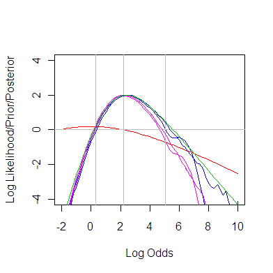
For this problem, using priors and elegant math from here and brute force numerical integration, we can show all inference pieces and their sum in one dimension for the log odds ratio parameterization for treatment effect.

The graph shows the LogPrior (red), LogIntegratedLikelhood (blue) and their sum the LogPosterior (purple) – just for the log odds ratio. Also a green curve for later. Their maximums have been arbitrarily set to 2 so that the horizontal line at 0 provides approximate credible interval.

plot2.pdf

Sorry I have yet to try this for (Pt-Pc) – probably doable by brute force – but log odds is a very convenient parameterization.

Now lets compare and contrast with the frequency approach.

In principle, the same integrated likelihood could be used – now just erase the LogPrior and LogPosterior. Then you go down about 2 units from the maximum of the LogLikelihood to get a approximate 95% confidence interval.
(Yes getting this just right, going down just the right distance and perhaps deviating the horizontal line from 0 degrees – such that it would have 95% coverage and this coverage is a constant function accross Pt and Pc is mathematically impossible but within any reasonable model uncertainty you can usually get close enough and always >= 95%)

The least wrong likelihood – that is just a function of log odds ratio – for this problem is the conditional likelihood (same math that gives the Fisher’s Exact test) and I should add that to the plot (it is not hard but not at hand right now)

The more general though a bit wronger approximation to the least wrong likelihood is the profile likelihood
– for each value of log odds ratio replace the unknown Pc with the mle for it and treat it as known. This traces out the peak over the surface in log odds direction and its known to approximate the conditional likelihood quite well. It is what drives logistic regression software and the _default_ in frequency based modelling.

That is added as the green curve in the plot above. It fails in the paired data case i.e. Neyman-Scott problems but otherwise works fairly generally.

Hopefully this shows why credible and confidence intervals will be very similar – in this problem. Both intervals mostly come from the blue/green curve (where they intersect the horizontal line).

This is a real simple problem – binary outcomes, two groups and randomized. Explaining this to people with little training is statistics – something I need to do soon – will likely be challenging.

Whats nice about the Bayesian approach here is that it can be displayed just using curves – for any parameter / parameterization one wants to focus on

– always using the same method. But there is actually no need to obtain the curves, one can grab a sample from the posterior surface and extract the posterior curve one wants to focus on.

On the other hand, one could use the profile likelihood in leu of the integrated likelihoods to get a approximate display – the error of thie approximation would show up in the difference between the extracted from the posterior surface log curve with the (marginal) LogPrior + LogProfileLikelhood curve.

But its also nice to show that the credible interval mostly comes from the peices that also provide confidence intervals and hence the confidence coverage should be pretty good (or maybe even better as in this example – Mossman, D. and Berger, J. (2001). Intervals for post-test probabilities: a comparison of five methods. Medical Decision Making 21, 498-507.)

Summary of an easy stats problem
Bayes: Grab posterior sample and marginalize to parameter of focus
Frequency: Marginalize the likelihood surface to something that is just a function of the parameter of focus – and do extensive math or simulation to get and prove its a confidence interval

Easy if both intervals mostly come from a log likelihood?

Question: Why don’t we give these picturesque descriptions of the workings of statistics to others?

K

Getting confidence into the scaffolding – even if Bayes did or did not intend that.

After noticing an event for my first stats prof

I made the mistake of downloading one of his recent papers

After suggesting that Bayes might have actually been aiming at getting confidence intervals – the paper suggests “Bayes posterior calculations can appropriately be called quick and dirty” means to obtain confidence intervals.

It avoids obvious points of agreement “There are of course contexts where the true value of the parameter has come from a source with known distribution; in such cases the prior is real, it is objective, and could reasonably be considered to be a part of an enlarged model.”

Uses an intuitive way of explaining Bayes theorem that I think is helpful (at least in teaching) “The clear answer is in terms of what might have occurred given the same observational information: the picture is of many repetitions from the joint distribution giving pairs (y1; y2), followed by selection of pairs that have exact or approximate agreement y2 = y2.obs, and then followed by examining the pattern in the y1 values in the selected pairs. The pattern records what would have occurred for y1 among cases where y2 = y2.obs; the probabilities arise both from the density f(y1) and from the density f(y2|y1). Thus the initial pattern f(y1) when restricted to instances where y2 = y2.obs becomes modified to the pattern f(y1|y2.obs) = cf(y1)f(y2.obs|y1)”

And (with added brackets) makes a point I can’t disagree with “conditional calculations does not produce [relevant] probabilities from no [relevant] probabilities.

Perhaps this is very relevant to me as I am just wrapping up a consulation where a 1,000 plus intervals were calculated and the confidence ones were almost identical to the credible ones – except for a few with really sparse data where the credible intervals were obviously more sensible.

But the concordance bought me something – if only not to worry about the MCMC convergence. (By the way these computations were made almost easy and fully automated by Andrew’s R2WinBugs package.)

The devil is in the details (nothing gets things totally right) – or so I am confident.

K

When experts disagree – plot them along with their uncertainties.

This plot is perhaps an interesting start to pinning down experts (extracting their views and their self assessed uncertainties) – contrasting and comparing them and then providing some kind off overall view.

Essentially get experts to express their best estimate and its uncertainty as an interval and then pool these intervals _weighting_ by a pre-test performance score on how good they are at being experts (getting correct answers to a bank of questions with known answers).

For those who are not familiar with consensus group work, a very good facilitator is needed so that experts actually share their knowledge instead of just personalities and stances.

The experts’ intervals could easily be plotted by their performance score, and weighting schemes of %correct, versus (%correct)^2, or ( (%correct)^2 or 0 if %correct< 50% ) considered. Better still - some data mining and clustering of experts' pre-test answers and best estimates. Note these could be viewed as univariate priors and points towards the much more challenging area of extracting, contrasting and combining multivariate priors. K

What’s most cool – the question mark in the name or the modelling of zombies?

Some recent interest has been raised by the following publication

zombies

by an seemingly unknown author – well not quite

Smith?

I have not had anything to do with predator/prey models since reading Gregory Bateson’s Steps towards an Ecology of Mind – but a question mark in one’s name – that just too cool to pass by!

K?

PS Favourite article title – also by Bateson with his daughter when she was a young child – “Why do French?”