Anders Huitfeldt writes:
Thank you so much for discussing my preprint on effect measures (“Count the living or the dead?”) on your blog! I really appreciate getting as many eyes as possible on this work; having it highlighted on by you is the kind of thing that can really make the snowball start rolling towards getting a second chance in academia (I am currently working as a second-year resident in addiction medicine, after exhausting my academic opportunities)
I just wanted to highlight a preprint that was released today by Bénédicte Colnet, Julie Josse, Gaël Varoquaux, and Erwan Scornet. To me, this preprint looks like it might become an instant classic. Colnet and her coauthors generalize my thought process, and present it with much more elegance and sophistication. It is almost something I might have written if I had an additional standard deviation in IQ, and if I was trained in biostatistics instead of epidemiology.
The article in question begins:
From the physician to the patient, the term effect of a drug on an outcome usually appears very spontaneously, within a casual discussion or in scientific documents. Overall, everyone agrees that an effect is a comparison between two states: treated or not. But there are various ways to report the main effect of a treatment. For example, the scale may be absolute (e.g. the number of migraine days per month is expected to diminishes by 0.8 taking Rimegepant) or relative (e.g. the probability of having a thrombosis is expected to be multiplied by 3.8 when taking oral contraceptives). Choosing one measure or the other has several consequences. First, it conveys a different impression of the same data to an external reader. . . . Second, the treatment effect heterogeneity – i.e. different effects on sub-populations – depends on the chosen measure. . . .
Beyond impression conveyed and heterogeneity captured, different causal measures lead to different generalizability towards populations. . . . Generalizability of trials’ findings is crucial as most often clinicians use causal effects from published trials (i) to estimate the expected response to treatment for a specific patient . . .
This is indeed important, and it relates to things that people have been thinking about for awhile recently regarding varying treatment effects. Colnet et al. point out that, even if effects are constant on one scale, they will vary on other scales. In some sense, this hardly matters given that we can expect effects to vary on any scale. Different scales correspond to different default interpretations, which fits the idea that the choice of transformation is as much a matter of communication as of modeling. In practice, though, we use default model classes, and so parameterization can make a difference.
The new paper by Colnet et al. is potentially important because, as they point out, there remains a lot of confused thinking on the topic, both in theory and in practice, and I think part of the problem is a traditional setup in which there is a “treatment effect” to be estimated. In applied studies, you’ll often see this as a coefficient in a model. But, as Colnet et al. point out, if you take that coefficient as estimated from study A and use it to generalize to study B, you’ll be making some big assumptions. Better to get those assumptions out in the open and consider how the effect can vary.
As we discussed a few years ago, the average causal effect can be defined in any setting, but it can be misleading to think of it as a “parameter” to be estimated, as in general it can depend strongly on the context where it is being studied.
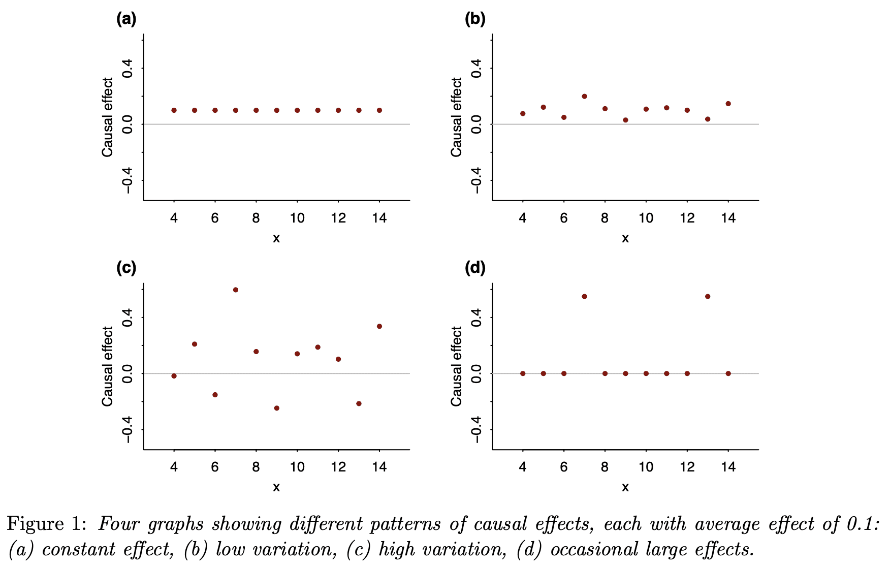
Finally, I’d like to again remind readers of our recent article, Causal quartets: Different ways to attain the same average treatment effect (blog discussion here), which discusses the many different ways that an average causal effect can manifest itself in the context of variation:
As Steve Stigler paper pointed out, there’s nothing necessarily “causal” about the content of our paper, or for that matter of the Colnet et al. paper. In both cases, all the causal language could be replaced by predictive language and the models and messages would be unchanged. Here is what we say in our article:
Nothing in this paper so far requires a causal connection. Instead of talking about heterogeneous treatment effects, we could just as well have referred to variation more generally. Why, then, are we putting this in a causal framework? Why “causal quartets” rather than “heterogeneity quartets”?
Most directly, we have seen the problem of unrecognized heterogeneity come up all the time in causal contexts, as in the examples in [our paper], and not so much elsewhere. We think a key reason is that the individual treatment effect is latent. So it’s not possible to make the “quartet” plots with raw data. Instead, it’s easy for researchers to simply assume the causal effect is constant, or to not think at all about heterogeneity of causal effects, in a way that’s harder to do with observable outcomes. It is the very impossibility of directly drawing the quartets that makes them valuable as conceptual tools.
So, yes, variation is everywhere, but in the causal setting, where at least half of the potential outcomes are unobserved, it’s easier for people to overlook variation or to use models where it isn’t there, such as the default model of a constant effect (on some scale or another).
It can be tempting to assume a constant effect, maybe because it’s simpler or maybe because you haven’t thought too much about it or maybe because you think that, in the absence of any direct data on individual causal effects, it’s safe to assume the effect doesn’t vary. But, for reasons discussed in the various articles above, assuming constant effects can be misleading in many different ways. I think it’s time to move off of that default.
The default assumption of a constant effect is also just a convenient computational shortcut in many cases – plug in a fixed value or estimate one parameter as opposed to many…
There is not a single new result on this paper… Morever, to give credit to Anders, he is selling himself short. Perhaps due to the convoluted language and notation used by the authors of the paper (which is a deficiency, and shows lack of understanding of the core principles), Anders fails to see that what they are doing is nothing but replicating the same things that have been said before.
Dear Jon,
Thank you for reading the article. I agree with your message on many aspects:
(1) I agree: Anders is selling himself short! We read, deeply appreciate, and found inspiration in Anders’ research work. As you can see, I quote him a lot. I hope this paper effectively conveys this and does it justice.
(2) What we say is indeed very coherent and consistent with some previous works. As the question is age-old, this is expected. And somehow the contrary would have been worrying.
We think that the formalism we proposed helps to propose contributions, for e.g. the link between generalization and collapsibility, link between a generative model and the causal measure that depends on the nature of the outcome (which we have not found written likewise. If we missed something, we would naturally correct and update our work right away!), the different choice of covariate set depending on the measure someone wants to generalize, the two identifications formula for generalization (e.g. Risk Ratio that does not appear a lot within the statistical community working on generalization).
Thanks again for your comment and remark.
(And I will answer to the whole post from Andrew Gelman and other comments ASAP :) )
I thought this was going to be a post on which summary statistic to use, another good topic (would be different for different policy decisions, different degrees of sophistication of reader).
Yes, I thought the same thing. It seems there is still a lot of disagreement about this.
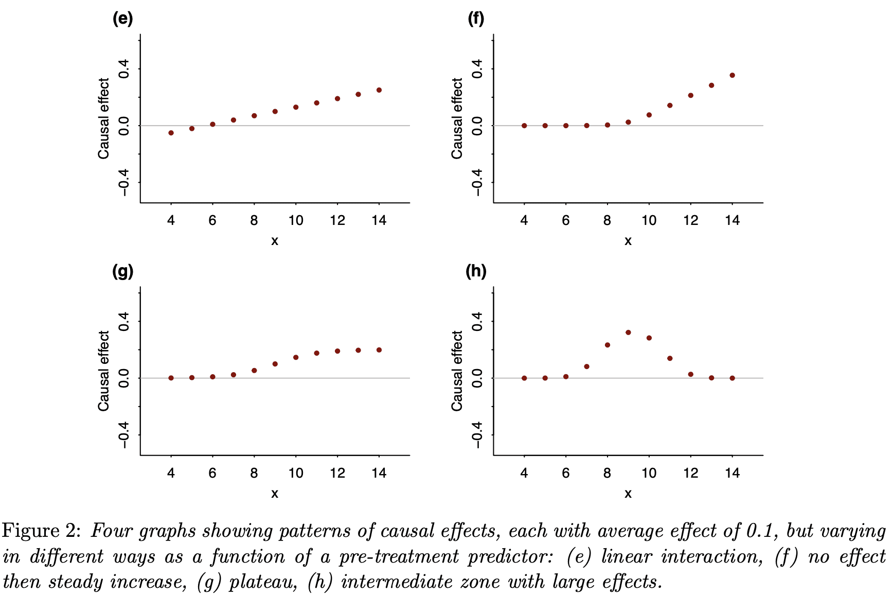
In your paper, you might note that 2e is the linear-no-threshold for harm from a treatment, and 2f is a threshold effect. I forget what lingo is used for 2g, the concave plateau effect. 2h is neat; the sweetspot effect arises in the context of a medicine where a moderate dose improves your condition but too much of anything becomes worse than the disease it is trying to cure.
Confused about “ So it’s not possible to make the “quartet” plots with raw data”. The graphs condition on a single x variable. Then treatment effect | x could empirically be assessed (count the deaths or the living) as the difference | x? Very similar to empirically assessing linearity in a covariate relation, where the covariate is associated with an outcome?
The impossibility of knowing an individual treatment effect comes in if we condition on multiple x. Similar to impossibility of learning the true model in prediction (“utopia”: https://pubmed.ncbi.nlm.nih.gov/26772608/ ).
So, causal inference and prediction may share the basic point of any estimate being a best guess?
You might be interested in this paper: https://www.ahajournals.org/doi/10.1161/HYPERTENSIONAHA.110.152421
The authors analysed blood pressure response in trials of one drug class (angiotensin converting enzyme inhibitors), and found that most of the between-person differences in short-term blood pressure change were attributable to noise in the outcome — a mixture of measurement error sensu stricto and short-term variation in blood pressure. They argue (I think correctly) that clinicians would often interpret these between person differences as differences in the causal effect of treatment, and that in this case they would be wrong. Some of the same people also looked at cholesterol-lowering treatment, with qualitatively similar conclusions. So there are settings in which people do look at differences in causal effect, and at least occasionally it’s actually true that the causal effect is relatively constant.
Since we were, at the time, looking for genetic influences on the effect of blood pressure drugs, the paper was a bit offputting — the less variation there is in the causal effect, the less room there is for important genetic causes of variation.
First and foremost, I would like to express my gratitude for your blog post. As a Ph.D. student, I feel tremendously honored by your interest in my work. It is truly rewarding to witness the scientific community engage in discussions about this topic. I would also like to extend my sincere appreciation to Anders, who generously shared this work. He is quite humble about his own contributions and overly generous in his praise of ours!
Your article raises many reactions & remarks to me.
Below are my two cents:
– About the [post](https://statmodeling.stat.columbia.edu/2009/07/31/estimating_trea/) discussing heterogeneity with Avi Feller and Chris Holmes, I agree with your thought-provoking notion of the ATE being a “dead end.” In fact, I sought to emphasize this very point in the notation section of my paper, where I discuss how causal effects reported in a RCT are intricately linked to the population (mathematically speaking through the expectation). I also appreciated the clarity with which you explained this concept in your paper on causal quartets: “Thinking about variation in treatment effects makes this clear: the average effect is not a general parameter; it depends on who is being averaged over.”
– After reading your blog post [The value of thinking about varying treatment effects: coronavirus example](https://statmodeling.stat.columbia.edu/2020/07/01/the-value-of-thinking-about-varying-treatment-effects-coronavirus-example/) : I perfectly agree that the average causal effect can be defined in any setting and has no reason to be a parameter of a model (of course, under some assumptions this can be the case. For e.g. this assumption I read a lot that the data generative model is something like Y = beta . X + A . \tau + epsilon, where \tau is directly the risk difference). What we try to highlight in our paper is that thanks to the binary nature of the treatment A, it is possible to write a generative model with no parametric assumptions. We simply decompose the outcome in a baseline part and a modifying part in the generative process (following Robinson’s work proposed in the 80’s for a continuous outcome). In your blog post, I really liked your remark about the “patient-mix”:
“Once we’ve accepted the idea that the drug works on some people and not others—or in some comorbidity scenarios and not others—we realize that “the treatment effect” in any given study will depend entirely on the patient mix. There is no underlying number representing the effect of the drug. Ideally one would like to know what sorts of patients the treatment would help, but in a clinical trial it is enough to show that there is some clear average effect. My point is that if we consider the treatment effect in the context of variation between patients, this can be the first step in a more grounded understanding of effect size.”
We indeed faced troubles to extend Robinson’s decomposition for a binary outcome. I have been taught at school that if I face a binary outcome, then I should use a logistic regression model. But I was really annoyed by the fact that the logistic model implies a complete interaction between all prognostic covariates, and one can no longer find something that would correspond to the intuition of a baseline risk and an effect.
This is how I came with the entanglement model, which sounds really more intuitive to me than the logistic model. In particular, the following quantity appears : `P(Y(1) = 1 | Y(0) = 0, X=x)` (or conversely `P(Y(1) = 0 | Y(0) = 1, X=x)` ). If I understand well your work, this corresponds to the idea of “a patient that would live either way” or “a patient that would die either way” or “a patient would be saved”. I think this could be the “underlying number” your are referring to as the treatment effect at the individual level.
Doing so, some of the causal measures only capture the “modification” and not the baseline part. If Y is continuous, the absolute difference does capture the modification and not the baseline. If Y is binary and the treatment effect is monotonous (harmful or beneficial for everyone) then the ratio — risk ratio or survival ratio — captures the above probabilities. Under such writing, some causal measures can be linked to a generative model, but not all of them.
– By the way, I would like to make an epistemological observation that I did not highlight in the paper. As a young statistician who has read both econometrics and clinical studies, I was quite surprised to discover that econometricians typically use the difference and clinicians the ratio when analyzing outcomes. This difference in approach may be attributed to the nature of the outcomes that each field focuses on. In economics, the outcomes of interest are usually continuous (e.g., prices, wages, and economic growth), whereas in medicine, binary outcomes are more common. As I developed these generative models, I was pleased to discover that they align well with existing practices in both fields. Moreover, I noticed that clinicians usually denote bad events with Y=1. This fits the idea of measuring the risk ratio, corresponding to `P(Y(1) = 0 | Y(0) = 1, X=x)` when taken with respect to x, which is the quantity that we are looking for when studying beneficial treatment. But taking the same measure for deleterious factor (for e.g. Y = thrombosis when A = oral contraceptive, leads to risk ratio above 1, which are entangled with the baseline and no longer corresponding to the probability of interest).
– I also completely agree that there is somehow nothing causal in our work. Interestingly, most of people (including me) are tempted to consider trial’s effect estimates as invariant because causal. This reminds me this Pearl’s quote (Causality, p.182 “Once people interpret proportions as causal relations, they continue to process those relations by causal calculus and not by the calculus of proportions”).
– Of course one can test for interaction or estimate the CATE using trial data. But sometimes this requires either modeling assumptions and/or a rather large sample size (see Gelman 2018a). This is usually not the case with RCT samples. This is why I am interested into generalization’s technics. Re-weighting a RCT could provide another answer, still thinking the effect as an average, but at least on the right target population of interest. In the end, policy makers are taking decision at the population-level, To me, generalization is a tool among others to help. I think this can also play the role of a sensitivity analysis. For e.g. if a trial’s effect is moving a lot when generalized to another population, then one can ask for more investigations before promoting the treatment as a new standard of care.
PS: My apologies for the delayed response. I am currently immersed in writing my Ph.D. thesis while simultaneously presenting at a conference last week. I perfectly knew that once I would start to deep dive in all the references and ideas your provide in this post, I would prefer thinking of all this rather than finishing to write my thesis chapter! :)