Part 1
Here’s the golf putting data we were using, typed in from Don Berry’s 1996 textbook. The columns are distance in feet from the hole, number of tries, and number of successes:
x n y
2 1443 1346
3 694 577
4 455 337
5 353 208
6 272 149
7 256 136
8 240 111
9 217 69
10 200 67
11 237 75
12 202 52
13 192 46
14 174 54
15 167 28
16 201 27
17 195 31
18 191 33
19 147 20
20 152 24
Graphed here:

Here’s the idealized picture of the golf putt, where the only uncertainty is the angle of the shot:
Which we assume is normally distributed:
And here’s the model expressed in Stan:
data {
  int J;
  int n[J];
  vector[J] x;
  int y[J];
  real r;
  real R;
}
parameters {
  real sigma;
}
model {
  vector[J] p;
  for (j in 1:J){
    p[j] = 2*Phi(asin((R-r)/x[j]) / sigma) - 1;
  }
  y ~ binomial(n, p);
}
generated quantities {
  real sigma_degrees;
  sigma_degrees = (180/pi())*sigma;
}
Fit to the above data, the estimate of sigma_degrees is 1.5. And here’s the fit:

Part 2
The other day, Mark Broadie came to my office and shared a larger dataset, from 2016-2018. I’m assuming the distances are continuous numbers because the putts have exact distance measurements and have been divided into bins by distance, with the numbers below representing the average distance in each bin.
x n y
0.28 45198 45183
0.97 183020 182899
1.93 169503 168594
2.92 113094 108953
3.93 73855 64740
4.94 53659 41106
5.94 42991 28205
6.95 37050 21334
7.95 33275 16615
8.95 30836 13503
9.95 28637 11060
10.95 26239 9032
11.95 24636 7687
12.95 22876 6432
14.43 41267 9813
16.43 35712 7196
18.44 31573 5290
20.44 28280 4086
21.95 13238 1642
24.39 46570 4767
28.40 38422 2980
32.39 31641 1996
36.39 25604 1327
40.37 20366 834
44.38 15977 559
48.37 11770 311
52.36 8708 231
57.25 8878 204
63.23 5492 103
69.18 3087 35
75.19 1742 24
Comparing the two datasets in the range 0-20 feet, the success rate is similar for longer putts but is much higher than before for the short putts. This could be a measurement issue, if the distances to the hole are only approximate for the old data.
Beyond 20 feet, the empirical success rates are lower than would be predicted by the old model. This makes sense: for longer putts, the angle isn’t the only thing you need to control; you also need to get the distance right too.
So Broadie fit a new model in Stan. See here and here for further details.
Shouldn’t the y-axis say “Frequency of success”?
“One-putt probability” is the same as “Frequency of success”
http://omega.math.albany.edu:8008/JaynesBook.html (Chapter 9)
For example, I can know someone is about to blow a foghorn just as the golfer is about to put. Then I would say the probability of success should be lower than the frequency. Even with no data on the effects of well-timed foghorns on putting (no idea of the frequency for that subset), we can give success a lower probability than the frequencies shown in the chart. Fisher makes a similar argument here: Fisher, R N (1958). “The Nature of Probability”. Centennial Review. 2: 261–274. http://www.york.ac.uk/depts/maths/histstat/fisher272.pdf
Also:
> set.seed(1234)
> rbinom(5, 1, .05)
[1] 0 1 1 1 1
Probability next number is a “success” = 0.5
Frequency of “success” = 0.8
Did you just logically equate “probability” and “frequency”?
You’re waving a red flag in front of a bull, right there…
Yes, you are correct. I was being very loose with the term ‘probability’. I should have used ‘one-putt frequency’.
I made a nice post (imo) with quotes/link from ET Jaynes and a reference to Fisher talking about it but looks like it got spambinned. Anyway, I find making the distinction helpful, but not important enough to attempt a repost.
Very cool! Is the Stan code for Broadie’s model somewhere? Did not see it in the links (pun intended)
Real world greens are not flat, so there is also the break to consider and it becomes more important for longer putts and depends on the particular green… We need info on this to fit a model including breaking
The best available data does not have (as far as I know) information about green contours. Just distances to the nearest inch or thereabouts.
I thought about that briefly and decided that the break was what a (good) golfer would take into account when deciding on the angle, so is already incorporated in the model, to a first approximation. Perhaps the standard deviation on the angle should increase with distance since the golfer has to decide on the angle rather than aim for the hole.
Sure, but with a flat green the question is how well can you estimate the angle at which the hole lies… a question of kinematics. With a sloped green it’s how well can you estimate the angle at which you should putt the ball so that dynamically it arcs into the hole… I think these are distinct skills, one is essentially measurement of angles the other is estimation of dynamical forces etc
I presented a paper at the Fields Institute Sports Analytics conference (joint work with Dongwook Shin) that showed the ranking of PGA Tour putters taking breaks and green contours into account was not very different than only using distance. Clearly uphill, downhill and sidehill puts are quite different in difficulty, but distance is the primary determinant of putt difficulty. Green contour effects average out over a larger number of putts because players tend not to have large systematic differences in the fractions of uphill, downhill and sidehill putts. There are significant systematic differences in the length of initial putts.
Curious if you interacted slope with length, it’s clear here that slope has to interact, it doesn’t really have a non-interacted effect
Presumably good golfers have more shorter putts than longer putts, bad golfers typically have more equal numbers of long putts and short putts.
While the ranking of players may not change when you use a more sophisticated model, I don’t think that is the question here. The question is whether the frequency of puts made is affected by break and other factors. I would be very surprised if break was not an important factor. I also strongly suspect downhill puts are much more frequently missed.
I imagine side-hill putts to be very difficult as well, you must putt somewhat uphill so that as the ball breaks downhill, it goes towards the hole, and the angle you have to putt is intimately connected with the speed you have to putt. Roughness of the green affects the speed, and that affects the direction as well. There are multiple solutions to the problem, just as for example you can throw a ball fast and hit a target on the ground, or you can lob it up in the air and hit a target on the ground, or anything in between if you keep the angle and the initial speed correct together. It gives you more options, but it can easily mean higher risk as well, if you miss your ball may roll downhill far from the hole. On a flat green if you miss but aren’t too far off, you’ll have a tap in at least.
It just seemed like an obviously interesting question to ask.
I think the model is par for the course!
This is a chip shot rather than a pure putt, but it’s a good example of what a golfer has to think about in terms of slope and speed of the green: Tiger Woods, 16th hole at 2005 Masters:
https://www.youtube.com/watch?v=DpRmF__A33U
That’s a fabulous example of what I’m thinking about. On a flat green, there is essentially only one direction to putt in, but on a contoured green direction is intimately connected to initial speed and the contour along the whole path. Strangely it can be the case that there are many ways to hit the ball into a contoured hole. That’s very obvious if you think about a drain at the bottom of a shower stall…
Given all these subtleties, it’s impressive how well a crude math/physics-based model can do. It’s like what Jaynes said: make some strong assumptions, then look at where the model does not fit the data and use this to motivate specific improvements to the model. Our version is slightly compared to what Jaynes could do because with Stan we can easily fit models with more free parameters, thus allowing more stages of this model-improvement iteration.
It’s a modern version of Lakatos/Kuhn normal science and scientific revolution, and we can do this in so many different application areas. Just amazing.
I feel lucky to have been an active researcher in the period during which these ideas became fully realized and part of statistical workflow rather than just implicitly visible in a few special examples (such as the Mosteller/Wallace Federalist Papers study, and whatever Turing et al. did to crack those codes).
Ahem…
What’s the prior for sigma ? Stan’s “default prior” ? Is this defensible ?
Emmanuel:
Sure, default models are defensible. Applied statistics is full of default models. Indeed, it would be difficult to find a statistical model that does not have any default components. You can start with all the linear and logistic regressions out there, etc etc. For any default model, it’s the usual story that we should be aware of ways in which the model can be improved.
P.S. Feel free to explain why you put “default prior” in quotes and why you wrote “ahem.” I feel like there’s something more you want to say, or something you’re implying, but I’m not quite sure what. I doubt you think that every part of every model, to be defensible, needs to be constructed completely from first principles. So I don’t think you could be opposed to defaults in general. Are there some defaults that are more bothersome than others?
> “Sure, default models are defensible.”
Of course. What I meant was “is this specific default model defensible in this particular case ?”.
>”Feel free to explain why you put “default prior” in quotes”
I wasn’t (and still am not) sure that this is the right term ; BTW, you use “default model” rather than “default prior”, and I’d nitpick that up to “default model part”…
>” and why you wrote “ahem.”
I thought that I might be underscoring an infelicious edit of the prior out of the model, hence apologizing for the inconvenience…
As for the notion of defaults : they are pertinent for a certain class of models and a certain class of problems. Using them in a given case entails to be able to defend their use in said case. That was what I meant.
My (non-)mastering of the goddamn’ English language might be responsible for the loss of meaning between what I intended and what you understood. Things might be easier if we both used, say, Latin, a non-mother tongue for al parties involvedf (and, BTW, one allowing for much more precision than the globish that passes for English in scientific communication…).
Emmanuel:
Je pense que la distribution a priori, c’est la partie le moins important dans ce modèle. Plus généralement, je pense que tout le monde regarde la distribution a priori avec bien souci mais moins regarder sérieusement le modèle pour les données. En ce cas, c’est clair à moi que la distribution a priori est moins important : on peut examiner la distribution a priori de sigma et voir qu’elle est très précis en comparaison à toute distribution a priori qu’est raisonnable.
Okay, you’re going to the idea of a low “relative weight” of the prior in the posterior (compared to the “high weight” of the data).
Doesn’t this legitimate a resurrection of the idea of using “part of” the data to choose a prior and the rest to estimate the posterior, or something like Zellner’s “g priors” ? The idea was enticing, but I don’t remember seeing used in a lot of applied papers…
ISTR that you used an idea close to that in the first edition of “Data Analysis Using Regression and Multilevel/Hierarchical Models” in order to show that some weakly informative priors “weighted” less than one observation (on having the book on hand, I can’t check that now).
BTW : if such “data-derived priors” stand to criticism, wouldn’t a tool more-or-less automating them be a valuable addition to Stan ?
It will be interesting to see how the statistics for 2019 will compare to prior years, as the new rules of golf, which went into effect on January 1, 2019, now allow for the flagstick to remain in the hole while putting from on the green. Previously, you could only do that if off the green (e.g. chipping).
The general consensus is that the proportion of putts that go into the hole from various distances will increase, since the flagstick will now serve as a backstop of sorts, allowing putts that would have previously skipped over the hole because they were going too fast, to go in. In fact, some professional golfers have specifically stated that they will now practice and judge putting speed based upon the ball going past the hole some distance, since they will now have an increased level of comfort that the flagstick will help in directing the ball into the hole.
> normal science and scientific revolution
I see it as just much better economy of research where most importantly getting less wrong is never blocked along with purposeful and continual attempts to maximize the expected rate of getting the less wrong.
I’m going to assume the data from 1996 and 2016-2018 are independent, and merge the datasets together, and run standard logistic regression on them. Is that using a Bayesian prior since it is using prior information? Or using a prior because I previously read another book on logistic regression? Couldn’t resist.
Summary:
-golfers predicted to miss more than make putts if distance > ~12ft
-prob(making distance=0 putt) = 94%. Maybe not 100% for small distances because of the well-known “yips”
-model over-predicts success for short distances, and under-predicts success for large distances
Now I’ll do the same thing, but if a distance is 16, I’ll merge those counts in with the distance 16.43 cases, etc., instead of treating them like separate categories. For example:
16 201 27
16.43 35712 7196
16.43 35913(=35712+201) 7223(=7196+27)
I wouldn’t have merged like this if it was 16.67. I would have merged that in with the 17 category. Dichotomania.
Doing that I get..not much changes at all from what I did at first.
Justin
http://www.statisticool.com
I realized there was a ton of overdispersion. So I refit with Williams’ method to accommodate it. Much better I think, but still not great.
Justin
http://www.statisticool.com
I may be making a fool of myself, but I’ll ask anyway.
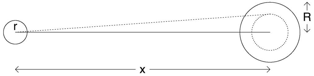
The golf ball is radius r. The hole has radius R. If the centre of the golf ball is within a distance of R from the centre of the hole, it is going to fall in. The Stan code above, and the description in Gelman and Nolan’s “Teaching Statistics” book (Section 9.3) assumes the ball falls in only if its centre is less than R-r from the centre of the hole. This views the golf ball and hole as two circles on the plane and requires that the smaller circle, with radius r, be fully enclosed by the larger one with radius R. But it seems obvious to me that all that is required is that the golf ball’s centre be within the larger circle, i.e. less than R from its centre.
If this is the case, the angle we are looking for is asin(R/x) and not asin((R-r)/x).
Of course, all of this just assumes the simple physical model, which of course could be expanded. But that’s another matter.
Mark,
First, you have a good point, thank you for noticing it. Nothing I say below should detract from that!
I’ve only golfed a handful of times, but even that has been enough to see the ball ‘lip out’ sometimes: if you hit the ball a bit ‘too hard’ — harder than it needs to in order to reach the cup — then even if the center of the ball is inside the edge of the cup, it can (and sometimes does!) escape. It happens more often than you might expect…well, certainly more obvious than you do expect, given that it’s “obvious” to you that it can’t happen at all! There’s a nice example at https://www.youtube.com/watch?v=oWqGRlq_wDg , it’s low-resolution but it’s good because the video is shot from directly behind the club so you can see the path of the ball quite well.
Anyway, you’re right that the simple model that they’ve assumed is deficient — and I congratulate you for noticing! — but the model you propose also misses a substantial real-world effect.