A bunch of us were arguing about how the Hamiltonian Monte Carlo step size should scale with dimension, and so Bob did the Bob thing and just ran an experiment on the computer to figure it out.

Bob writes:

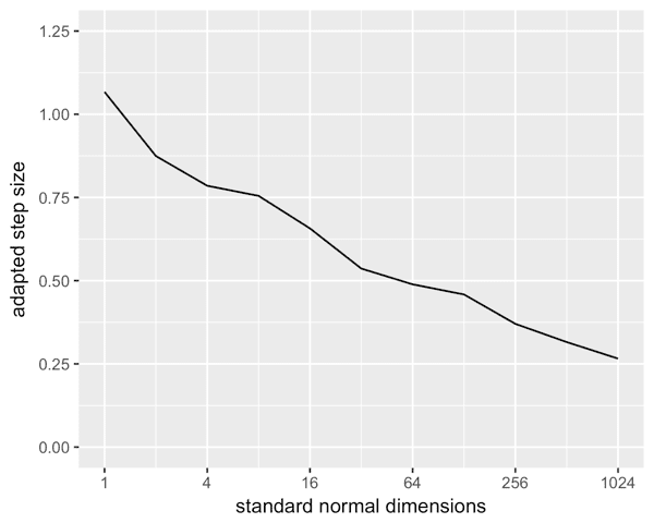
This is for standard normal independent in all dimensions. Note the log scale on the x axis. The step size declines but not nearly as sharply as 1 / sqrt(N), which would have the 1024 dimensional about 1/10th what it actually is.

He continues:

HMC isn’t like Metropolis. It’s not just these step sizes, but also the gradient that adjusts the momentum and the fact that momentum behaves like momentum. The gradient used to update momentum keeps the Hamiltonian trajectory running through the typical set even with fairly large step sizes. This is what Betancourt refers to as “flow” in his intro to HMC.

Here’s the R code to make the above graph:

mas <- function(fit) {
  sampler_params <- get_sampler_params(fit, inc_warmup = FALSE)
  return(c(sampler_params[[1]][1000, 2],
           sampler_params[[2]][1000, 2],
           sampler_params[[3]][1000, 2],
           sampler_params[[4]][1000, 2]))
}

library(rstan)
model <- stan_model(model_code = "data {  int N; } parameters { vector[N] alpha; } model { alpha ~ normal(0, 1); }")

K <- 11
stepsizes <- rep(0, K)
for (N in 1:K) {
  fit <- sampling(model, data=list(N = 2^(N - 1)), refresh = 0)
  stepsizes[N] = mean(mas(fit))
}

for (k in 1:K) {
  print(sprintf("N = %5d;  step size = %4.2f",
                2^(k - 1), stepsizes[k]),
        quote=FALSE)
}

library(ggplot2)
plot <-
  ggplot(data.frame(dimensionality = 2^(0:(K - 1)),
                    stepsize = stepsizes)) +
  geom_line(aes(x = dimensionality, y = stepsize)) +
  scale_x_log10(name = "standard normal dimensions",
                breaks = c(1, 4, 16, 64, 256, 1024)) +
  scale_y_continuous(name = "adapted step size",
                     limits = c(0, 1.25),
                     breaks=c(0, 0.25, 0.5, 0.75, 1, 1.25))
plot
ggsave("std-norm-stepsizes.png", width = 5, height = 4)