Milad Kharratzadeh shares a new case study. This could be useful to a lot of people.
And here’s the markdown file with every last bit of R and Stan code.
Just for example, here’s the last section of the document, which shows how to simulate the data and fit the model graphed above:
Location of Knots and the Choice of Priors
In practical problems, it is not always clear how to choose the number/location of the knots. Choosing too many/too few knots may lead to overfitting/underfitting. In this part, we introduce a prior that alleviates the problems associated with the choice of number/locations of the knots to a great extent.
Let us start by a simple observation. For any given set of knots, and any B-spline order, we have: $$ \sum_{i} B_{i,k}(x) = 1. $$ The proof is simple and can be done by induction. This means that if the B-spline coefficients, $a_i = a$, are all equal, then the resulting spline is the constant function equal to $a$ all the time. In general, the closer the consecutive $a_i$ are to each other, the smoother (less wiggly) is the resulting spline curve. In other words, B-splines are local bases that form the splines; if the the coefficients of near-by B-splines are close to each other, we will have less local variability.
This motivates the use of priors enforcing smoothness across the coefficients, $a_i$. With such priors, we can choose a large number of knots and do not worry about overfitting. Here, we propose a random-walk prior as follows: $$ a_1 \sim \mathcal{N}(0,\tau) \qquad a_i\sim\mathcal{N}(a_{i-1}, \tau) \qquad \tau\sim\mathcal{N}(0,1) $$
The Stan code,
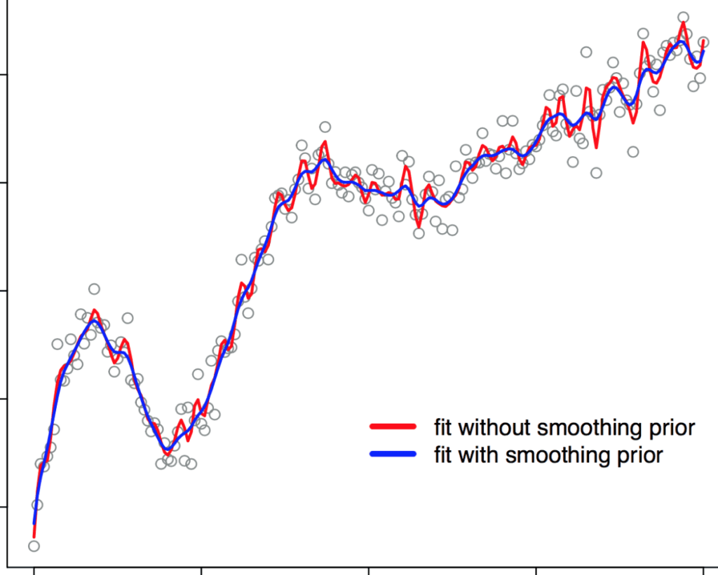
b_spline_penalized.stan, is the same as before except for thetransformed parametersblock:transformed parameters { row_vector[num_basis] a; vector[num_data] Y_hat; a[1] = a_raw[1]; for (i in 2:num_basis) a[i] = a[i-1] + a_raw[i]*tau; Y_hat = a0*to_vector(X) + to_vector(a*B); }To demonstrate the advantage of using this smoothing prior, we consider an extreme case where the number of knots for estimation is much larger than the true number of knots. We generate the synthetic data with 10 knots, but for the Stan program, we set the number of knots to 100 (ten times more than the true number). Then, we fit the model with and without the smoothing prior and compare the results. The two fits are shown in the figure below. We observe that without using the smoothing prior (red curve), the large number of knots results in a wiggly curve (overfitting). When the smoothing prior is used (blue curve), we achieve a much smoother curve.
library(rstan)
library(splines)
set.seed(1234)
num_knots <- 10 # true number of knots
spline_degree <- 3
num_basis <- num_knots + spline_degree - 1
X <- seq(from=-10, to=10, by=.1)
knots <- unname(quantile(X,probs=seq(from=0, to=1, length.out = num_knots)))
num_data <- length(X)
a0 <- 0.2
a <- rnorm(num_basis, 0, 1)
B_true <- t(bs(X, df=num_basis, degree=spline_degree, intercept = TRUE))
Y_true <- as.vector(a0*X + a%*%B_true)
Y <- Y_true + rnorm(length(X), 0, 0.2)

num_knots <- 100; # number of knots for fitting
num_basis <- num_knots + spline_degree - 1
knots <- unname(quantile(X,probs=seq(from=0, to=1, length.out = num_knots)))
rstan_options(auto_write = TRUE);
options(mc.cores = parallel::detectCores());
spline_model<-stan_model("b_spline.stan")
spline_penalized_model<-stan_model("b_spline_penalized.stan")
fit_spline<-sampling(spline_model,iter=500,control = list(adapt_delta=0.95))
fit_spline_penalized<-sampling(spline_penalized_model,iter=500,control = list(adapt_delta=0.95))
Yessssssssss!
P.S. No cat picture. Cos this stuff is just too damn important.
Very interesting case study! I think it is worth mentioning that the brms and rstanarm packages (both based on Stan) offer quite general support for splines leaving the technicalities of the data preparation to the mgcv package.
The brms package is PHENOMENAL.
This is great, thank you for posting. These appear to be ‘p-splines’ — is that correct?
Looks great. Does anyone have experience/intuition about when it is better to use splines and when Gaussian process regression?
I have worked with both in brms and it seems as if splines can be used with far greater data sets, since computing the covariance matrix for Gaussian processes becomes increasingly complicated for more data points.
I just started a fork (https://github.com/mike-lawrence/Splines_in_Stan) that includes comparison against a GP. As Paul says, GPs are much more computationally costly, so it takes longer but does better at recovering the true function than even the penalized splines, which are still too wiggly.
Cubic splines have a nice interpretation that makes them popular in functional data analysis: They can be viewed as the solution to a least squares problem (with smoothness constraints) for data lying in a Hilbert space. They’re also generally very fast — I routinely deal with datasets containing tens of thousands of curves, all of which need to be smoothed and interpolated, and using Gaussian process just isn’t feasible, even though they tend to be more “expressive”. It’s also easy to take derivatives of splines, which I need to do often.
There’s also a huge amount of work on spline linear/regression models, which helps. Fitting similar models using GPs would probably need A) custom programs, and B) lots of computer time.
Nicely done! Splines are really under-appreciated for how expressive they can be as model components.
Thanks for this useful post. I am currently working to fit a Bayesian GAM model with autoregressive errors in STAN. This example fits a univariate P-spline in stan, I am wondering can we also fit a P-spline modelling interactions which can be approximated by the tensor product of one dimensional P-spline?
Stan Totally not ANacronym
Very cool. I do a lot with functional data, so finally seeing a spline implementation in Stan is great. I’ve extended it a little bit to a functional regression model for fixed-effects with separate smoothness penalties, though it’s not very well optimized.
https://github.com/areshenk/splinyStanSplines
Hey Corson,
thanks very much for your model with the fixed-effects! Do you have any idea how to combine the splines with random effects instead of the fixed ones? You would be a great help.
Thanks in advance,
Joline
Joline, just to make sure, do you mean random effects particular for the spline coefficients? If so, what about using a multivariate normal prior for the spline coefficients with an unstructured variance-covariance matrix (potentially working with LKJ priors over correlation matrices)? Or what about using a hierarchical Gaussian Process prior for spline coefficients, where the first level would explain fixed effect spline coefficients and the second level group specific deviations? Haven‘t seen this anywhere, though…
I’ve been wanting to better understand splines and GP recently, but couldn’t find any approachable online resources for it. Anyone have recommended resources for understanding splines and/or GPs?
For splines in the broader context of functional data analysis, I can’t recommend Ramsay and Silverman’s “Functional Data Analysis” enough.
For GPs, if the written material that comes up when Googling “Gaussian process tutorial” isn’t approachable, maybe try some youtube videos…?
What is the practical difference between this and:
http://jofrhwld.github.io/blog/2014/07/29/nonlinear_stan.html?
Besides (potentially) having far fewer parameters, using a spline basis allows you to easily enforce all kinds of useful properties. Want your estimate to be periodic? Use a Fourier basis. Want it to be monotonic? Use a monotonic basis. Positive? Constrain the basis coefficients to be positive. Want to guarantee that your estimate has a continuous derivative up to n-th order? No problem, B-splines can do that easily.
If you have prior information about smoothness, why not just use fewer knots?
For anyone (like me) who wants to use this, I _think_ there is a subtle bug in the prior for a[1] (if anyone else can check that would be great!). See https://github.com/milkha/Splines_in_Stan/issues/6
I _think_ there is a subtle bug in adding the intercept twice, namely here:
Y_hat = a0*to_vector(X) + to_vector(a*B);
and in bs( … , intercept = TRUE)
This is a very helpful post, great work by Milad. I am working on implementing P-splines in RStan, P-splines as proposed by Eilers and Marx (1996) that penalize second-order differences. The results by just applying `mgcv::gam(log(Y) ~ s(X, bs = “ps”)` is different from the effect achieved by using random-walk prior. How should I adjust the example to do a (simple) penalized spline regression? I am new to the Bayesian framework and would like to seek help. Any advice is appreciated.