The above is the question asked to me by Michael Stutzer, who writes:
I have attached an increasingly influential paper [“Effects of Adolescent Caffeine Consumption on Cocaine Sensitivity,” by Casey O’Neill, Sophia Levis, Drew Schreiner, Jose Amat, Steven Maier, and Ryan Bachtell] purporting to show the effects of caffeine use in adolescents (well, lab rats anyway) on biomarkers of rewards to cocaine use later in life. I’d like to see a Gelmanized analysis of the statistics. Note, for example, Figure 2, panels A and B. Figure 2, Panel A contrasts the later (adult) response to cocaine between 16 rats given caffeine as adolescents, vs. 15 rats who weren’t given caffeine as adolescents. Panel B contrasts the adult response to cocaine between 8 rats given caffeine only as adults, vs. 8 rats who weren’t given caffeine. The authors make much of the statistically significant difference in means in Panel A, and the apparent lack of statistical significance in Panel B, although the sign of the effect appears to still be there. But N=8 likely resulted in a much larger calculated standard error in Panel B than the N=16 did in Panel A. I wonder if the results would have held in a balanced design with N=16 rats used in both experiments, or with larger N in both. In addition, perhaps a Bonferroni correction should be made, because he could have just lumped the 24 caffeine-swilling (16 adolescent + 8 adult) rats together and tested the difference in the mean response between them and the 23 adolescent and adult rats who weren’t given caffeine. The authors may have done that correction when they contrasted the separate Panels differences in means (they purport to do that in the other panels), but the legend doesn’t indicate it.
Because the paper is getting a lot of citations, some lab should try to replicate all this with larger sample sizes, and perturbations of the experimental procedures.
My reply:
I don’t have the equipment to replicate this one myself, so I’ll post your request here.
It’s hard for me to form any judgment about the paper because all these biology details are so technical, I just don’t have the energy to track everything that’s going on.
Just to look at some details, though: It’s funny how hard it is to find the total number of rats in the experiment, just by reading the paper. N is not in the abstract or in the Materials and Methods section. In the Results section I see that one cohort had 32 adolescent and 20 adult rats. So there must be other cohorts in the study?
I also find frustrating the convention that everything is expressed as a hypothesis test. The big big trouble with hypothesis tests is that the p-values are basically uninterpretable if the null hypothesis is false. Just for example:
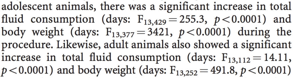
What’s the point of that sort of thing? If there’s a possibility there is no change, then, sure, I can see the merit of including the p-value. But when the p-value is .0001 . . . c’mon, who cares about the damn F statistic, just give me the numbers: what was the average fluid consumption per day for the different animals? Also I have a horrible feeling their F-test was not appropriate, cos I’m not clear on what those 377 and 429 are.
I’d like to conclude by saying two things that may at first seem contradictory, but which are not:
1. This paper looks like it has lots of statistical errors.
2. I’m not trying to pick on the authors of this paper. And, despite the errors, they may be studying something real.
The lack of contradiction comes because, as I wrote last month, statistics is like basketball, or knitting. It’s hard. There’s no reason we should expect a paper written by some statistical amateurs to not have mistakes, any more than we’d expect the local high school team to play flawless basketball or some recreational knitter to be making flawless sweaters.
It does not give me joy to poke holes in the statistical analysis of a random journal article, any more than I’d want to complain about Aunt Edna’s sweaters or laugh at the antics of whoever is the gawky kid who’s playing center for the Hyenas this year. Everyone’s trying their best, and I respect that. To point out statistical errors in a published paper is not an exercise in “debunking,” it’s just something that I’ll notice, and it’s relevant to the extent that the paper’s conclusions lean on its statistical analysis.
And one reason we sometimes want brute-force preregistered replications is because then we don’t have to worry about so many statistical issues.
I found reading the paper frustrating. This is the kind of thing where the results should be summarized in one or two graphs and be convincing. Looking at the graphs, that’s definitely not the case in this paper. Figure 2 panel a vs b shows essentially no difference between adolescent caffeine vs adult caffeine. The only difference is whether or not the differences between water/caffeine were or were not statistically significant.
Panel c&d the same kind of thing is happening. They’re taking a statistical significant difference between water and caffeine for the adolescent group, and lack of such statistical significance in the adult group, as evidence that the cocaine response is different between the adolescent and adult group. If you look at just the two cocaine bars and their “half-sided” error bar, you could guess that maybe there’s no statistical significant difference between cocaine@adolescence – cocaine@adult, or even if there is a statistically significant difference, so what, show me the practical effects.
again, in panel e vs f. Just look at the black-dot curves, is there any practical significant difference between those curves? Again, the difference between statistically significant and not significant is not itself statistically significant.
The bit that amuses me about these sort of studies is the level of nested surrogacy. i.e. the degrees of indirection from the actual effect anyone cares about.
e.g. Lab rat to human extrapolation ; “bio-markers for rewards of cocaine use” etc.
Even if the effect were real (which I doubt it is), it’d be quite the stretch to the situation we are really interested in.
The other thing to look out for in studies like this is the dosage. Here it looks like 25-35 mg/kg of caffeine each day for a month (28 days). For a 80 kg human that would be like 2400 mg of caffeine a day, using 150 mg of caffeine per cup of coffee* would give 16 cups of coffee a day.
Also, remember these are rats with much shorter lifespans than humans. The adolescents and adults only lived 82 and 121 days respectively, corresponding to living 34 and 23 percent of their lives drinking 16 cups of coffee a day.
*http://coffeefaq.com/site/how-much-caffeine
The headline claim from the abstract:
“these findings suggest that caffeine consumption during adolescence produced changes in the NAc that are evident in adulthood and may contribute to increases in cocaine-mediated behaviors.”
To show this there would be a plot, and some kind of analysis, of “changes in the NAc” vs “cocaine-mediated behaviors”. They actually do not show the evidence in favor of their primary finding in this paper. It isn’t clear whether the histology was done on the same rats that were tested behaviorally:
“Seven days following caffeine consumption (adolescent studies: P62 or adult studies: P101), rats were killed by rapid decapitation and bilateral 1mm3 tissue punches were taken from chilled tissue slices containing the NAc and the caudate–putamen.”
If it was the same rats, they have no excuse for not plotting histology vs behavior. If it was not the same rats, they need to explain why they couldn’t collect both types of data from the same rats. I don’t see that anywhere but maybe missed it.
Also, look at how the upper y axis limits are chosen for figure 1 so as to make it impossible to tell what is going on, very annoying. Another odd thing is that the caption of fig 2 says “sub-threshold dose of cocaine (7.5 mg/kg)”, but they go on to use 5 mg/kg for the microdialysis study shown in figure 3.
I bet it’s the same rats, it would be a lot of work for no purpose to grow up additional rats and give them caffeine etc and then not measure their behavior and just sacrifice them for histology. So, let’s say it really is the same rats. Why did they not scatter-plot the cocaine behavior scores against the “NAc” measurement for each individual? One thing I think is clear with this stuff is that typically histology is hard to quantify. not impossible, but it takes a lot better understanding of quantification techniques than is typical in a biology lab (I’ve worked with biologists to do this kind of stuff).
Just plotting Locomotor vs Cocaine dose, scatter-plot with two colors (for each dosing regime), and a LOESS curve. Literally, one line in ggplot:
ggplot(data,aes(x=Cocaine,y=Locomotor,color=DoseRegime))+geom_point()+stat_smooth();
Nope, found it (in a weird place):
“Behavioral measures, tissue collection, and microdialysis studies were performed in separate cohorts of animals.”
It is difficult for me to understand why behavior would be incompatible with the other methods. Maybe the microdialysis caused too much damage for the histology, but behavior should be compatible with both. Apparently this was done at University of Colorado Boulder. I downloaded the “Animal Use Protocol Application Form” from here: http://www.colorado.edu/vcr/iacuc/forms-glossary-additional-resources
I see in section 7.2 that the researchers agreed to:
“List measures you will take to ensure that pain, distress, discomfort and injury will be limited to that which is unavoidable in the conduct of scientifically sound research.”
I was thinking the AAALAC accreditation of the university may be in danger:
“The 2011 Guide specifies that the Committee is obliged to weigh study objectives against animal welfare concerns in accordance with the tenets of the Three R’s [Replace, Reduce, Refine] . This analysis is typically already performed by IACUCs in their reviews of proposed animal studies. AAALAC International expects that IACUC’s (or comparable oversight body), as part of the protocol review process, will weigh the potential adverse effects of the study against the potential benefits that are likely to accrue as a result of the research. This analysis should be performed prior to the final approval of the protocol, and should be a primary consideration in the review process. For animal use activities potentially involving pain and/or distress or other animal welfare concerns, the AAALAC International site visitors will assess how the Committee conducts this analysis.”
http://www.aaalac.org/accreditation/faq_landing.cfm
However, interestingly it turns out they are not accredited:
“Is CU-Boulder AAALAC accredited?
Not yet, but that is our ultimate goal. Soon, AAALAC will be invited to reveiw our animal care program.”
http://www.colorado.edu/vcr/oar-animal-resources/oar-frequently-asked-questions
Also, I realized what they did isn’t really histology. For some reason I thought they were quantifying a stain, instead they did western blots on homogenized tissue samples…
I agree that a study with larger N would be a good thing here in the abstract, but on the other hand, why should we waste money on something that is super weak and not well modeled?
The first step here would be to get the actual datasets, and re-do this analysis with at least the proper things being compared: compare the cocaine response of adolescent cohort to the adult cohort directly. Don’t compare the statistical significance of the adolescent cocaine vs water to the statistical significance of the adult cocaine vs water!!!
This book might be relevant to this discussion (not read):
“Statistics Done Wrong, And How To Do Better” by Alex Reinhart https://www.sciencebasedmedicine.org/statistics-done-wrong-and-how-to-do-better/
+1 especially for the conclusion.
I think a big problem with statistics in other scientific fields is that so many non-statistical scientists are being forced to spend so much time learning statistics, which takes away from the time the can spend doing the actual science of their field. And it’s my thought that the worst scientific conclusions are made from pure trust in misguided statistical procedures; would himicanes have ever been published if the hypothesis were judged more on merit than GoFP’ed p-values?
Not to say a scientific world without statistics is the solution. But there is a real cost in trying to force every biologist to be a statistician.
I agree with your concerns about the study in question, but I cannot agree with your emboldened sentence about P-values: “The big big trouble with hypothesis tests is that the p-values are basically uninterpretable if the null hypothesis is false.” I reckon that you have expressed one of the things that you call a zombie idea.
That sentence implies that P-values are in some manner more interpretable when the null is true. In what way? I can only assume that people who make such statements are thinking about the probability interpretation of P-values which has to be couched in terms of “assuming the null is true”. However, that cannot be the basis of your claim because even when the null hypothesis is false the P-value retains that probability interpretation–the assumption is built in and it is explicitly an assumption rather than an assertion about the real world.
Despite the zombie, P-values are readily interpreted when the null is false: the further the observed effect size (scaled) is from the null hypothesises effect size the smaller the P-value will be for a given sample size according to the statistical model. That makes the P-value a straightforward index of the discrepancy when the model is acceptable. It presents no interpretative challenge beyond its non-linear relationship with effect size and sample size, and neither of those challenges is relieved in the circumstances where the null hypothesis is true.
P-values do not communicate the observed effect sizes sufficiently conveniently to obviate the need for the effects to be explicitly stated and shown. However, that is true when the null is true or false. The utility of the discrepancy interpretation of P-values is dependent on the appropriateness of the statistical model, but, again, that is the case when the null is true or false.
The interpretative mine-field of P-values is the same when the null is true or false. You should kill the zombie.
Michael I am confused.
> non-linear relationship with effect size and sample size
If there is no effect and those myriad of other assumptions are fine (e.g. no selection, proper randomization, etc.) then the distribution of p_values will be Uniform(0,1) – invariant to sample size (unless very small and discrete) and invariant to the form of no effect.
And the more difficult question of what to make of a reported value, when one knows the distribution they are being drawn from is Uniform(0,1) is absolutely nothing – all p_values are equally likely.
Keith, you are looking from the wrong direction. The P-value is not trying to communicate anything about itself, but rather information about the relationship between the observed data and the parameter(s) of the model that is used for the test.
If the null is false then, yes, the distribution of P-values is uniform, but if the null is false then the distribution is non-uniform. But that is not what matters. What does matter is that small P-values are more common when there is an effect size different to the null hypothesis. The smaller the P-value the more that data support parameter values that differ from the null.
You don’t need to know the distribution of P-values implied by the true effect size in order to interpret the P-value.
Michael:
No, it is not true that “the smaller the P-value the more that data support parameter values that differ from the null.” Unless you use this as your definition of “support.”
Andrew: Could you give an example of a situation where, everything else being equal, the smaller the p-value wouldn’t correspond to higher support against the null? Or do you mean that the p-values in different situations are not comparable?
Carlos:
What is meant by “everything else being equal”? When I see p-values in research articles, I don’t see everything else being equal. What I see is passages such as quoted in the above post.
I see no point in explaining to you what “ceteris paribus” means in this context. But I don’t understand what does it have to do with the fragment you included in your post. I thought your point was that one knew in advance that the rats would gain weight, especially the younger ones, so the result as presented was not interesting. Maybe you would have prefered that they just said “as we can see in charts 1 (c),(d),(g),(h) there is a clear trend of gaining weight and increasing fluid consumption as the experiment progresses and the rats keep growing” without giving a p-value. But I don’t see how giving it would be a “statistical error”: the small p-value is indeed what you would expect if there is a clear trend, a trend which is highly unlikely to happen from natural variability alone if the rats were not actually growing. (I don’t know how it was calculated, though, maybe they are doing it wrong somehow.)
Is the definition of “everything else being equal” substantive to the question at hand?
If we get stuck on that definition a lot of the typical reasoning used in science would be stymied.
Rahul:
It’s no big deal, but I can’t really respond to this person’s question if I don’t understand what he is asking!
Andrew: I thought it was a rhetorical question, but if it is not the case I can explain what I meant. Everyhting being equal is to be understood here as “all the assumptions made to calculate a sampling distribution remain unchanged.” You are doing the same experiment, in the same way, with the same rats, everything is the same as far as the calculcation of a p-value under the null hypothesis is concerned but you obtain a different outcome. Imagine in one case you get p=0.0001 (there is a clear trend in chart 1d) and in another you get p=0.3 (there is no apparent trend in the chart). The former scenario seems to support the idea that rats get fatter (i.e. the null hypothesis “rats don’t gain weight” is false) more than the latter. Maybe you can give an example where the p-value for outcome A is lower than for outcome B and it doesn’t indicate a higher support for the null hypothesis being false when the outcome is A rather than B.
Carlos:
Sure, but that’s not what’s being done. Nobody’s comparing 2 experiments on the same rats. Rather, some rats are being compared to other rats. In that case what I find relevant is a comparison to the variation between rats, not a comparison to a distribution under a null hypothesis that makes no sense. I just don’t see the relevance of this particular comparison.
Andrew: maybe we don’t disagree, but it’s hard for me to tell because I’m having some difficulty to follow the discussion. Michael Lew was not comparing some rats to other rats in the comment you replied to. The fragment of the paper included in your post is not comparing some rats to other rats. Now you may be talking about the issues that Michael Stutter mentions about Figure 2. I agree that panel A and panel B don’t seem very different and maybe with more data there would be separation in the curves. But this is a different subject entirely.
Andrew, you will need to supply a bit more detail before I can understand what you might be alluding to. I think that you might be wrong.
Michael, I will not claim that you are wrong but I am still confused.
I am not confused about nominal definitions of p_values (e.g. information about the relationship between the observed data and the parameter(s) of the model that is used for the test) but rather what to make of a p_value so “that fruitful reasoning can be made to turn upon it, and that it can be applied to the resolution of difficult practical problems” as Peirce put it.
> The smaller the P-value the more that data support parameter values that differ from the null.
Well given all the needed assumptions are know to hold, yes some parameter values but not all.
> You don’t need to know the distribution of P-values implied by the true effect size in order to interpret the P-value
But you claimed “smaller the P-value the more that data support…” so you need some sense of that distribution and if as sometimes is the case its almost uniform – the connection between smaller and more would be very weak (and as we don’t know the true effect size we never know when).
Also, at least with a single isolated study, we should always be very unsure that the needed assumption hold adequately.
>Well given all the needed assumptions are know to hold, yes some parameter values but not all.
Yes and no. The P-value is, just as a likelihood function and therefore and Bayesian analysis model-bound. So is a frequentist dichotomisation into significant or not significant. The support given by a P-value for inference concerning the parameter of interest is always subject to the caveat “according to the chosen model”. Thus in circumstances where the model is inappropriate the message that might be taken from the P-value might inherit that inappropriateness, but so would the message from any other statistical summary.
>some parameter values but not all.
True. I agree. However, it need not be all parameter values for my assertion to be correct. I did not intend it to entail all values of the parameter. If you want to see which values are well supported and which are not well supported then the likelihood function is what you want. (As Corey mentions below, the P-value and model and sample size together entail the relevant likelihood function.)
>But you claimed “smaller the P-value the more that data support…” so you need some sense of that distribution and if as sometimes is the case its almost uniform – the connection between smaller and more would be very weak (and as we don’t know the true effect size we never know when).
Consider the circumstance where you have calculated a single P-value from an experiment where you are confident that the statistical model is appropriate. Say you observe a P-value of 0.02. You know then that the model fits the observed data less well when the parameter of interest is set to the null hypothesised value than when it is set to a range of alternative values. It is still possible that the null is true, because data are somewhat misleading quite often, but you cannot know its truth without a god-like viewpoint. Thus when you say that the distribution of the P-values _might_ be uniform, I cannot say you are wrong, but the P-value of 0.02, (i.e. greater than 0.015 and less than 0.025) is more likely to have come from a distribution where values in that range are more common. You don’t need to know which particular distribution of P-values pertains to know that the observed P-value of 0.02 lends support to parameter values other than the null. (The relevant likelihood function will show which particular parameter values that are better supported than the null.)
Keith, let’s say we’re not questioning the model, which is normal, unknown mean and unknown variance. I hand Michael the likelihoodlum a sample size and an observed p-value and say, “Okay, smart guy, infer something!” Here’s what (I’m pretty sure) he does: he writes down the density of the p-value as a function of the unknown mean μ (or equivalently, he backs out the observed t statistic value and uses the density of the non-central t distribution) and then shows me a plot of the likelihood function of μ. As a Bayesian, I have to say this seems eminently reasonable to me.
This isn’t quite right — we can use the p-value to do likelihood inference on the ratio of the unknown mean to the unknown standard deviation, which is proportional to the non-centrality parameter μ.
Right, so you are being stuck with someone else’s choice of parameter of interest and distributional assumptions but with absolutely no ability to assess the assumptions.
The confidence distribution folks have the problem when they try to invert from the confidence distribution to get a pseudo-likelihood to use in meta-analysis.
I don’t disagree, and I think Michael admits as much in his original post; I just wanted to point out that the likelihoodist account does actually do something to address this concern of yours: “you need some sense of that distribution and if as sometimes is the case its almost uniform – the connection between smaller and more would be very weak”. Under the assumption that the model is good enough, the likelihood function quantifies exactly how weak.
Keith, an inability to reconstruct the data in sufficient detail to perform a different analysis using a different model or test statistic is not a special feature of P-values. If you see it as a weakness then it is a weakness of most (maybe all) statistical approaches. I think that overloading an evidential summary with the responsibility to communicate everything about the data for every purpose is unhelpful.
> If you see it as a weakness
No, I was simply replying to a possibility that Corey raised though I was surprised he raised it as until then there was no mention of likelihood anywhere in the post or any of the comments.
But then in your comment below you indicate your earlier comments do involve your likelihood paper somehow.
Still do not think that answers the questions I raised but maybe they were not really relevant.
Missed your answers above.
If we think the null hypothesis is false to begin with, then a p value like 0.05 can actually provide evidence *for* the null hypothesis. Suppose that you have two models, the “non-null” model and the “null” model. Suppose that your non-null model predicts data which would have p = 1e-17, but in fact you get p=0.05.
There are only 2 models, so
p(Null Model | T(Data))+ p(Non Null Model | T(Data)) = 1
p(Null Model | T(Data)) = 1 – p(Non Null Model | T(Data)) = 1-p(T(Data) | Non Null Model) p(Non Null Model) / p(T(Data))
p(Non Null Model) is large because we assume probably the null is false, p(T(Data)) is smallish but not as small as p(T(Data) | Non Null Model) because it includes the possibility of the null. So we wind up with something like 1 – x where x ~ p(Non Null Model | T(Data))/p(T(Data)) is still small.
so with a proper calculation following the logic of cox’s axioms, because you get p = 0.05 it’s pretty certain that the null is true.
Note, I realize that in most null hypothesis testing situations the “non null model” is just “the parameter is anything other than 0” but in realistic inference we should do a better job than testing “exactly 0” against “not zero” holding some distribution of outcomes assumed constant and ignoring all other explanations except that some particular parameter might vary across the whole real line.
Daniel, where you write “there are only 2 models” you are working in a mental model that differs from mine in an important way. You are seeking a decision between two hypotheses, whereas I am trying to estimate the value of the parameter of interest. I have one model but an infinite set of values of the parameter of interest. Which of those values are better supported by the data? The P-value doesn’t tell me directly which values are best supported, but a (one-sided) P-value that differs from 0.5 tells me that the null hypothesised value of the parameter is not as well supported as some other values. Whether the difference in support is enough for me to make a decision is not the issue at hand, and neither is the fact that a likelihood function would communicate the relative levels of support far better than the P-value.
It seems odd to me that you would try to impose a dichotomising approach when we are discussing the evidential interpretation of P-values.
The dichotomization approach is really just a for-instance to show how data values that give low p values for one model can actually imply that that model is the correct model depending in part on how likely those data values are under other plausible models. We can easily embed the same thing in a continuous model.
The big problem with p values is that they’re intentionally ignoring everything but the null model, whereas proper inference should be Bayesian inference according to Cox’s theorem where all plausible models are considered simultaneously. People either need to deny some of Cox’s assumptions and explain why that makes sense, or just stop using p values in the way they are typically used.
Daniel, I think that you are mistaken, or you have a different interpretation of values of the parameter from mine. If a one-sided P-value from a model with a single continuous parameter is less than 0.5 then there is a value of the parameter that is better supported by the data than the null hypothesised value. Yes? In that case I don’t see how you are thinking to “embed the same thing in a continuous model”.
Second, the P-values are often said to “ignore everything but the null” but that is not quite true. They are anchored to the null, but the model that yields the P-value also yields a likelihood function on all values of the parameter. That means that the P-value points to the likelihood function which means that the P-value encodes information regarding values of the parameter other than the null. The conventional dichomising viewpoint ignores that information, but it is available nonetheless. (See Corey’s comments above about the likelihood function, or my arXived (rejected) paper: https://arxiv.org/abs/1311.0081).
RE: “People either need to deny some of Cox’s assumptions and explain why that makes sense”, there is plenty of room to do this, or at least to deny some of the supposed implications, and people have done so explicitly.
There are also a number of arguments that weren’t developed specifically to address Cox’s approach but which could be converted into such arguments.
It’s still an interesting thought experiment to me, though, so I do think it has value.
As a challenge, here is an alternative thought experiment/challenge – try to give some of your own reasons for disagreeing with Cox (and/or Jaynes)!
I have yet to see anything convincing against the Cox approach. There are a few technical arguments, things about discrete spaces, and about the non-zero derivative of the conjunction function, and whatnot, but those aren’t fundamental denials of the basic concepts. What have you seen where people outright deny the basic axioms such as consistency with boolean logic (ie boundedness of the plausibility) or whatever? Everything I’ve seen is about technical issues that have not been convincing to me.
Probably not the place to discuss here.
I would just ask – which presentation of Cox’s argument do you take as canonical? Jaynes’ maybe? What exactly do you take Cox/Jaynes to show? I think even the answer to this last question would raise plenty of debate.
Do you think e.g. Gelman’s approach conforms to the Cox/Jaynes axioms? Why/why not?
In terms of Jaynes’ presentation I think I could probably personally fairly easily doubt (and I think point to some arguments against) Desideratum (I) and Desideratum (IIIb), both in their necessity and in their specific formalisation. In both a ‘practical’ and a ‘philosophical’ sense. I also think there are at least reasonable cases to make against the use of Boolean logic in the sense it’s employed by Cox/Jaynes.
In terms of the technical conditions I’m not sure what the current status of e.g. differentiability requirements is and to what extent these rule out/in different approaches. These might also raise some concerns to me, but I couldn’t say of the top of my head. (And if the fix was e.g. nonstandard analysis then this would raise further questions!)
Which is not to say that it isn’t an interesting model for thinking about ways of formalising ‘reasonable’ reasoning.
I just find it important to make a distinction between ‘here is a reasonable argument for/illustration of why this approach might be reasonable’ and ‘here is a argument with *obvious premises* that *must* be accepted and which lead to the *only* way of thinking about this topic’. I’m happy to accept the former, sceptical of the latter.
More importantly, I’d be interested in the possibility of you putting forward your own counterargument – e.g. imagine you had to take part in a formal debate or something – where might you start?
Perhaps you could write a blog post some time and we could continue discussion there.
The best overview I’ve seen on cox’s theorem is this:
http://ksvanhorn.com/bayes/Papers/rcox.pdf
Which has a back-and forth associated as well, you can see here:
http://ksvanhorn.com/bayes/papers.html
I think he goes through a bunch of the technical bits that people have objected to, but I don’t see any of that as anything like convincing for why *scientist* trying to determine what ideas are most compatible with reality as shown in data should adopt any other system.
Happy to oblige with a blog post if you promise to look for it. It will be a while though (maybe a month or two) due to some high priority issues I’ve got going on.
Mean time, take a look at the Van Horn article I think it renders the fat out of the issue so that what’s left is pretty minimal.
Sure :-)
Van Horn’s presentation is interesting. I’ve briefly seen the article before but never properly read it.
Reading it a bit more carefully, it occurs to me that with his (subtle) modifications there actually isn’t much conflict between various schools of inference, e.g. Bayesian, Likelihood and Frequentist. But perhaps that is a topic for another day.
I ran up a blog post on Van Horn’s article with a little commentary, just so we could have a place to talk about it, not much that I’m actually adding, more like just discussing what he says. See what you think.