In response to some of the discussion that inspired yesterday’s post, Gary McClelland writes:
I remain convinced that discretizing a continuous variable, especially for multiple regression, is the road to perdition.
Here I explain my concerns. First, I don’t buy the motivation that discretized analyses are easier to explain to lay citizens and the press. Second, I believe there is an error in your logic for computing the relative efficiency for splitting into three groups. Third, and most importantly, dichotomizing or trichotomizing two or more continuous variables in a multiple regression is an especially bad idea. In such cases, the loss of efficiency is irrelevant because the discrete predictor variables have a different correlation than the continuous variables. As a consequence, the parameter estimates from the discrete analysis are biased. I’ll explain all three issues in some detail.
1. I just don’t buy the motivating issue—that the essence of a regression analysis can’t be explained to lay people. Explaining a regression result in terms of differences between averages is fine with me, but that doesn’t require a dichotomized analysis. We assume there is some true population difference between the average case in the top group (whether that be the top half, top third, top 27%, top quarter) and the average case in the bottom group. Let’s call those two population means muH and muL (for high and low). Our goal is to estimate that population mean difference. We, as statisticians, have two (at least) ways to estimate that mean difference muH – muL.
a. We do the split and compute the corresponding averages ybarH and ybarL and our estimate of muH – muL is ybarH – ybarL.
b. We regress y on x, as originally measured, to obtain yhat = b0 + b1 x. then we estimate muH – muL using (b0 + b1 xbarH) – (b0 + b1 xbarL) = b1(xbarH – xbarL).
Both are unbiased estimates of muH – muL and both can be described as “our data estimates the difference between the average person in the top group in the population and the average person in the bottom group in the population is …” The only difference between the two methods is that the variance of the estimate in (a) is greater than the variance of the estimate in (b). That implies that there will be many times when the estimate in (a) is either higher or lower than the estimate in (b). Hence, the two analyses will seldom agree on the magnitude of the raw effect. That gives researchers another degree of freedom to report the estimate that better fits their argument. We should use the the more precise regression estimate (b) and explain it in terms of a mean difference between high and low groups. If we are communicating to a lay group we should give them our best estimate and that is b1(xbarH – xbarL). We don’t need to explain to them how we got our estimate of muH – muL unless they ask. and even then the explanation isn’t that difficult. “We compared our prediction for a person with an average score in the top group to our prediction for a person with an average score in the low group.”
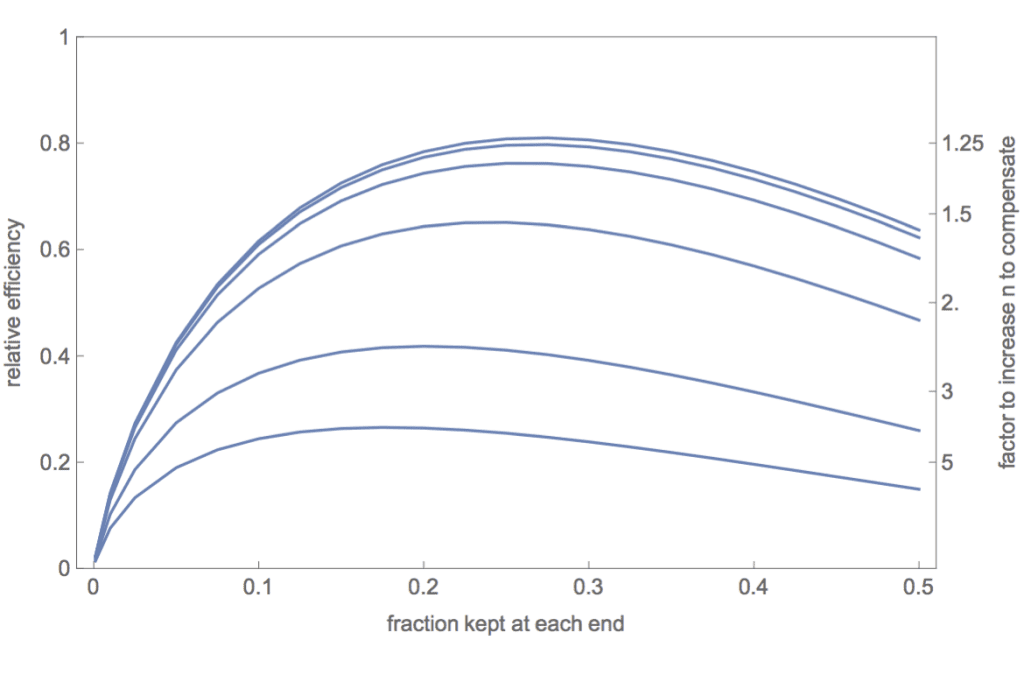
2. Using extreme groups in a three-way split of a single continuous predictor: The error in your mathematical analysis, I believe, is the assumption that the residual variance remains constant and is therefore the same in Eq. 4 and Eq. 5 in Gelman & Park (2008). It is easy to disprove that assumption. The residual variance is V(e) = V(Y)(1-r^2). Discretizing changes the correlation between X and Y. Furthermore, restricting the values of Y to cases that have extreme values of X will necessarily increase the V(Y). The exception is that when r = 0, V(Y) will be unchanged. Hence, your claims about the relative efficiency of extreme groups apply if and only if r = 0. In an attached Mathematica notebook (also included the pdf if you don’t use Mathematica) and an attached R simulation file, I did a detailed analysis of the relative efficiency for different values of b in the model Y = b X + e. This graph summarizes my results:
The curves represent the relative efficiency (ratio of the variances of the estimates of the slopes) for, top to bottom, slopes of b = 0, .25, 0.5, 1, 2, and 3. Given the assumption that V(e) = 1 in the full data, these correspond to correlations, respectively, of r = 0, 0.24, 0.45, 0.71, 0.89, and 0.95. The top curve corresponds to your efficiency curve for the normal distribution in your Figure 3. And, as you claim, using an extreme group split (whether the keep fraction is 0.2, 0.25, 0.27, or 0.333) is superior to a median split at all degrees of relationship between X and Y. However, relative efficiency declines as the strength of the X,Y relationship increases. Note also that the optimal fraction to keep shifts lower as the strength of the relationship increases.
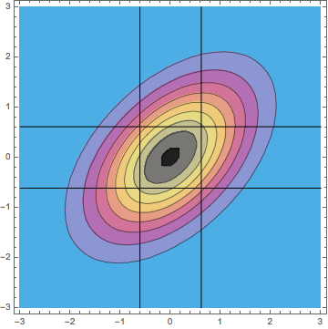
Are these discrepancies important? For me and my colleagues in the social sciences, I decided the differences were of interest to geeky statisticians like you and me but probably not of practical importance. Within the range of most social science correlations (abs(r) < 0.5), the differences in the efficiency curves are trivial. And if a social scientist felt compelled for reasons of explainability to discretize the analysis, then I certainly agree that doing an extreme-groups analysis is preferable to doing a median split. However, if a researcher studying a physical industrial process (where the correlation is likely very high and high precision is desired) were tempted to do an extreme-groups analysis because it would be easier to explain to upper management, I would strongly advise against it. The relative efficiency is likely to be extremely low. On the right axis I’ve indexed the factor by which the sample size would need to be increased to compensate for the loss of efficiency. The price to be paid is extremely high. 3. When two or more correlated variables are analyzed via multiple regression, discretizing a continuous variable is a particularly bad idea not only because of reduced efficiency, but more importantly because discretizing changes the correlational structure of the predictors and that leads to bias in the parameter estimates. Most of the discussion in the set of median split papers in JCP concerned whether one could get away with splitting a single continuous variable which was to be analyzed in multiple regression with another continuous variable or as a covariate in an ANCOVA design. We thought both the considerable loss of power and the induced bias as a function of the predictor correlation were adequate reasons to reject such dichotomizations. I will be interested to see what your take is on that. However, I believe that doing an analysis with two discretized variables, whether by median splits or by “thirds” is a terrible idea because of the bias it induces. For median splits of two predictors with a bivariate normal distribution with correlation rho = 0.5, I can show analytically that the correlation between the dichotomized predictors will be 0.33, resulting in a confounding of the estimated slopes. Specifically, b1 = (5 b1 +b2)/6 and b2 = (b1 + 5 b2)/6. That is not good science. In the case of trichotomizing the two predictors and then using the extreme four corners of the 3 x 3 cells, I can show analytically that the predictor correlation INCREASES from 0.5 to 0.7. You can see why the correlation is enhanced in the bivariate distribution with correlation rho = 0.5 in this contour plot:
Using only the four extreme cells makes the correlation appear stronger.
I haven’t yet worked through analytically the bias this will cause, but I have experimented with simulations and observed that there is an enhancement bias for the coefficients. If one coefficient is larger than the other, then the value of the larger coefficient is unbiased but the value of the smaller coefficient is increased (i’ve been working with all positive coefficients). For example, when predictors x and z are from a bivariate normal distribution with correlation 0.5 and the model is y = x + 2 z + e, then the cut analysis yields coefficient estimates of 1.21 and 2.05. The 21% enhancement of the smaller coefficient isn’t just bad science, it isn’t science at all. The source of the problem can be seen in the comparison of two tables. The first table is the predicted means using the regression equation for the full model applied to the actual cell means for x and z.
-3.7 1.2
-1.2 3.7The following table is the mean y values for each cell (equivalently, the model derived from the cut variables).
-4.0 1.0
-1.0 4.0In other words, the cut analysis exaggerates the differences in the cell means. This arises because the cut analysis forces a false orthogonal design. This is confounding in the same sense that bad experimental designs confound effect estimates.
A particularly disturbing example is for the model y = x + 0*z + e, the coefficients for the cut analysis are 0.96 and 0.11, a spurious effect for z. This can be seen in the table of means for the four groups:
-1.3 -1.1
1.0 1.3In fact, the columns should have been identical as in
-1.22 -1.23
1.22 1.21consistent with the null effect for z. This spurious effect is akin to the problem of spurious effects due to dichotomizing two variables identified by Maxwell & Delaney (1993).
In short, discretizing two continuous predictors has no place in the responsible data analyst’s toolbox. At the end of section 2.8 you describe doing the appropriate full analysis as an option. I strongly disagree this is optional—it is a requirement.
You present bivariate analyses across years both for a continuous analysis (Figure 5) and an extreme-groups analysis (Figure 6). If both ways of estimating the effects were unbiased and equally efficient, we would expect the rank order of a given effect across years to remain the same as well as the rank order of the three effects for a given year to remain constant. Neither seems to be the case. The differences are not large relative to the standard error so perhaps these differences are just due to the increased variability of the discretized estimates. However, if religious attendance and income are correlated and especially if the degree of this correlation changes over the years, then I suspect that some of the differences between Figures 5 and 6 are due to bias induced by using discretized correlated predictors. I think the logits of Figure 5 transformed back to probability differences would have been more appropriate and no more difficult to explain.
I also am attaching a 5th paper in the JCP sequence—our effort at a rebuttal of their rebuttal that we posted on SSRN.
For the quick version, here’s McClelland’s note, which begins:
Gelman & Park (2008) argue that splitting a single continuous predictor into extreme groups and omitting the middle category produces an unbiased estimate of the difference and, although less efficient than using the continuous predictor, is less destructive than the popular median split. In this note I show that although their basic argument is essentially true, they overstate the efficiency of the extreme splits. Also their claims about optimal fractions for each distribution ignores a dependency of the optimal fraction on the magnitude of the correlation between X and Y.
In their Equations 4 and 5, Gelman & Park assume that the residual variance of Y is constant. It is easy to show that is not the case when discretizing a continuous variable, especially when using extreme groups. . . .
I don’t have time to look at this right now, but let me quickly say that I prefer to model the continuous data, and I consider the discretization to just be a convenience. I’ll have to look at McClelland’s notes more carefully to see what’s going on: is he right that we were overstating the efficiency of the comparison that uses the discretized variable? Stay tuned for updates.
P.S. I don’t want to make a big deal about this, but . . . this is the way to handle it when someone says you made a mistake in a published paper: you give them a fair hearing, you don’t dismiss their criticisms out of hand. And it’s more than that: if you have a reputation for listening to criticism, this motivates people to make such criticisms openly. Everybody wins.
I would have to do some digging, but if my (very old) memory serves Tukey in one of his EDA books suggests dividing variables into three parts in regressions as a way to have a resistant regression. He gives some reasoning for the recommendation, but I don’t remember them. I believe the same idea is in one of Mosteler’s books.
You are probably referring to Tukey’s 1978 chapter in a collection of survey-related topics dedicated to Hartley. The short 7-page chapter is titled, “The Ninther, a Technique for Low-Effort Robust (Resistant) Location in Large Samples.” The relative efficiency of Tukey’s method for normally-distributed data was 55%. It did better against thick-tailed distributions. But his main motivation for suggesting the technique was to be able to do something for “impracticably large datasets” which he considered to be datasets with more than a million observations. If he had had modern computing, it seems unlikely he would have suggested such a technique. There is a good discussion of Tukey’s ninther method in this bloc: http://www.johndcook.com/blog/2009/06/23/tukey-median-ninther/
For an explanation of the “three-group resistant line” from exploratory data analysis (including background), see
John D. Emerson and David C. Hoaglin, Resistant Lines for y versus x, pages 129-165 in Understanding Robust and Exploratory Data Analysis (D. C. Hoaglin, F. Mosteller, and J. W. Tukey, eds.). John Wiley & Sons, 1983 (Wiley Classics Library edition, 2000).
If you are trying to convince people who would be skeptical of your statistical estimates, then it may be more convincing if you supplement your analysis with a pooled analysis. In those circumstances a median split pooling is probably more convincing, as there are fewer choices for the investigator to make. I used this approach in two papers where i argue for global warming leading to more and stronger hurricane surges.
http://www.glaciology.net/Home/Miscellaneous-Debris/moreandstrongerhurricanesurges
I put the observational record and pooled stats in paper1, and the model fit in paper2.
A number of things are often glossed over in debates of this sort in the social sciences:
1. The assumption of continuity for variables generated via ordered categorical processes and for which small variations cannot be shown to be theoretically meaningful.
2. The definition of bias put forth by McClelland is grounded in the assumption that the *correct coefficient* results from math that assumes a normally distributed continuous variable and any variation from this equals bias.
3. The use of sample distribution metrics rather than theoretically meaningful categorizations — when the sample distribution does not cover the full range of possible values (as is often the case in reasonably small sample studies using college students) it is not possible to test whether a linear or curvilinear model would better represent the theoretical relationship at the population level. In this case a median split compares only sample specific high vs. low values. With large enough representative samples this is not an issue, but that is so uncommon in the social sciences that it is an issue far more often than acknowledged.
I think this is a bit unfair. McClelland is using a bog-standard model as a test bed in which to examine the performance of the trichotomized estimator; I don’t think he’s putting forth a claim that his definition of bias holds in full generality.
Thanks Corey! Yes, I just used bivariate normal as an example. I believe the bias will apply to any bivariate distribution. A key issue in any multiple regression analysis is the correlational structure of the predictor variables. Even if you don’t start with an a priori theoretical distribution and just work with the sample at hand, discretizing two predictors will change their correlation. I can’t prove this, but my experience is that on average dichotomizing will decrease the predictor correlation and produce estimates that are a weighted average of what the coefficients would have been in the continuous analysis. Trichotomizing and using all three groups also decreases the predictor correlation, leaving out the middle group will increase the correlation. It is easy to construct examples where these changes in the correlational structure will create an effect in the discrete analysis when there is absolutely no effect in the continuous data. Whatever the underlying distribution, discretizing two or more predictor variables in multiple regression analyses cannot be good science.
Gary:
Would you agree that whether creating discrete groups is better or worse for any particular situation is an empirical question that can be tested via sensitivity analysis on multiple repeated future data collections?
Well, I’m always open to empirical demonstrations. But there is strong statistical theory and simulations that show, except for a few chance events now and then, the continuous analysis is better than using discrete groups both in terms of precision (smaller standard errors) for univariate analyses and accuracy (no bias) for multivariate analyses. If someone were to propose such a study, I’d advise them to find something else more productive to study. But perhaps I haven’t quite understood your question.
I am arguing that the assumptions of this type of analysis are not generalizable to certain types of psychological constructs and that these situations are not members of the set “chance events now and then”. I am further saying that for these types of constructs it is the framing of the analysis that is problematic including the notion that the correlation at the continuous level of predictor and outcome variables is not the appropriate standard against which to make the judgment of better or worse. And that a sensitivity analysis would serve as a better alternative because its assumptions are not confounded with the assumptions of the mathematics being challenged. I am also saying that I developed something like this in which the theoretically derived categories outperformed multiple regression models consistently, across time, and with far less shrinkage than the empirically derived predictive regression models on psychological variables assumed to be continuous and am thus fairly confident in my assertion. Though it is always possible that my findings were the result of multiple false positives in favor of my hypothesis and thus further empirical testing is always warranted.
I also think you are minimizing the implications of this for some areas of psychometrics if this hypothesis is true. I spent a little time last night in R messing around with how I might be able to simulate an appropriate data set and will let you know when I do.
Can somebody elaborate on what “small variations cannot be shown to be theoretically meaningful” means?
What is the counter-example? When can small variations be shown to theoretically meaningful? What is the “theory” one uses to establish meaningfulness?
Small variations in length can shown to be important within certain contexts. Whereas small variations in a psychological construct cannot be shown to be similarly meaningful. A difference between a 4.2 and 4.3 on an summated or averaged scale of items does not result in consistent variations in predictions of behavioral outcomes.
Correction: Small variations in length can be shown to be important within certain contexts.
Isn’t that a case to case decisions?
e.g. If I am estimating GIS Car Journey times the difference between 4.2 miles and 4.3 miles is probably not meaningful either. But it doesn’t mean that Geo-analytics algorithms concerned benefit by working on binned data rather than continuous variables.
You can always coarse-grain your final output or predictions.
The distance has a meaning in and of itself that can be precisely defined. How is that comparable?
We can both agree that the difference between 4.2 and 4.3 miles = 0.1 miles and we can identify the time with which it takes to travel that far based on a variety of variables. The same is not true of a psychological construct.
Yes, but there’s pesky things like measurement errors and least counts. When your GIS algorithm throws up 4.2 miles and 4.3 miles what accuracy was the map coded with.
If the distance concerned is the trip to the two nearest Walmarts do I measure till the parking lot or the check out lane.
All I’m saying is that there are all kinds of issues even in non-Psych settings that can make small differences vague and not meaningful. That by itself does not seem a good argument in favor of binning a perfectly good continuous variate.
Yes, but the binning in your GIS example is being done with a reasonable amount of precision and measurement error reasonably normally distributed. Whereas the binning process with psychological scales moves from these direct binning processes with consistent measurement errors to measurement error that includes things such as the summation of items with disparate meaning, differing perceptions which may be directly related to the construct under study, etc. Your examples are not related to the measurement of distance itself.
Most psychological constructs are not continuous in any real world sense and treating it as such simply because we assign numbers to it and say so does not change this reality.
A point of clarification:
The examples you provided are related to applying the measurement of distance to the real world and not about the measurement of distance itself, a problem that has been solved, that is truly continuous, and that can be applied with a great deal of precision in some settings.
The challenges of accurate measurement of distance in some settings does not change the nature of distance, the fact that there is no ambiguity about the meaning of .01 miles even though there may be ambiguity in whether or not it is possible to actually travel that distance given obstacles.
This same cannot be said of .01 empathy.
Moreover, a difference of 1 in measuring a psychological construct may not mean the same thing at different parts of the scale (e.g., the difference between 4 and 5 may not mean the same as the difference between 3 and 4), whereas a difference of one mile does mean the same thing, whether it’s between 4 miles and 5 miles, or between 3 miles and and 4 miles.
Ok, but how would discretizaton help with this issue?
The point is that the types of measures often used for psychological constructs (e.g., scales 1,2,3,4,5) are already discrete. So methods that assume a continuous variable are questionable.
Well, obviously if your original measurement was indeed discrete then it makes perfect sense to stick to those bins.
I don’t think anyone is arguing in favor of converting (say) a 5-class scale into an artificially continuous variable.
The question is when dealing with something like income or IQ or age or voting percents whether to discretion them.
Andrew:
In what way is discretization a convenience? i.e. In what sense is a continuous variable inconvenient?
Rahul:
When writing Red State Blue State, I wanted to write things such as, Richer people vote 15 percentage points more Republican than poorer voters. Rather than saying that the logistic regression coefficient of voting on income was whatever. Or, even worse, just saying that voting predicts income and stopping there. I wanted to engage the non-statistically-expert reader in the data so that he or she could evaluate my claims directly. I was trying to avoid the “Freakonomics” approach in which the author just feeds conclusions to the reader, without the reader being able to engage with the data.
Doesn’t defining “richer” vs “poorer” leave open a lot of author degrees of freedom?
Rahul:
I used upper third and lower third as recommended in our paper. In any case, what’s important here is transparency.
But can’t such statements still be easily derived from regression coefficients? I.e., Gary’s whole point #1? In general what is your response to point #1?
Jake:
Fitting the regression model and then summarizing by derived quantities is just fine—indeed, that’s exactly what I would do if I needed to fit a model with any complexity. But sometimes we can make the direct comparison between upper and lower third, and that’s evan simpler. Simplicity has some value in communication.
Also there’s the point that some people want to use discrete categories. If you’re going to use discrete categories and take differences or run regressions, I think it makes sense to use 3 categories rather than 2.
I wonder if Evan Simpler would agree that he’s a direct comparison between upper and lower third.
Hey—it’s good to know that at least one person is reading these blog comments!
I think that discretisation is a reasonable thing in cases in which the exact numerical value suggests a precision that doesn’t exist or isn’t meaningful in practice. This depends on the application. I just saw somebody a few days ago who asked me about data that was about the time point at which a certain electrodiagnostic signal starts and the time point at which a certain physical action starts, for which they had some measurements. They were basically interested in whether the electrodiagnostic signal would happen (more or less) reliably before the physical action. They extracted these “starting times” by some dodgy algorithm from fairly complex curves and this algorithm quite obviously had some issues. At times it would locate the starting time at some meaningless crazy place because of some nonstandard feature of the curve. They wanted to analyse the time differences taken as continuous and I suggested to reduce these to binary data “electrodiagnostic signal comes first yes or no”. Voila, no issues with normality and outliers anymore, and they measure the thing of most direct interest, namely the percentage with which things happen in the right order.
The thing here was that a) they were essentially interested in a binary feature of in principle continuous data and b) there were good reasons to mistrust the precision in the continuous measurements. In these circumstances, why not?
By the way, I don’t deny that given some time some interesting things could be found looking at the continuous results, and of course one could wonder whether they could find something to more reliably measure the times, but this is not a real collaboration, rather people turning up and asking for help who don’t have the time and money to do (or pay somebody for) more sophisticated things.
> I don’t deny that given some time some interesting things could be found looking at the continuous results
Maybe in the distant future but for the near future all (recorded) results are to finite precision.
The real issue here (though not likely the practical issue) seems to be one of variable systematic error in the extractions rather than truncation to finite precision (and your solution seems to amount to qualifying those systematic errors as not being large enough to more than rarely change the sign.)
They may change the sign occasionally, but when data are discretised this will just make the probability for “correct order” closer to 50% (and increase its variance), which I think is appropriate. No sophisticated outlier handling needed.
I wonder if I’m alone in feeling that this discussion is…well, it’s definitely not so pointless as to be silly, but… somewhat in the direction of silly. Two bins, three bins, four bins, five bins…there’s nothing wrong with any of these. “In the top quintile of income, x% of voters chose the Democrat; in the lowest quintile it was y%.” That’s fine. Use deciles if you want. Or talk about the preferences of the one-percenters versus everybody else. It’s all fine when it comes to _presenting_ the results.I agree with Andrew that non-statisticians find this to be much easier to understand than regression coefficients.
When it comes to _analyzing_ the results you should use a better model if you have one. Maybe that’s a regression model.
If you have limited time and you realize you’re not going to have time to analyze the data one way and present the results another way, then OK, pick 3 or 4 bins, that’s going to be fine most of the time.
On the subject of measuring distances, I’ll never forget taking a land surveying class at Laney College (because I needed it, but it wasn’t offered at UC Davis in the semester I needed to take it). The class was taught by a very good surveyor, but it was the first time he’d taught it, and the instrumentation was, I kid you not, manufactured in about 1910. He brought in some professional computerized equipment for one day to verify some of the work we’d done.
So, we’re doing a survey traverse of some concrete nails we’d put in place (using powder-driven nails, which caused the Oakland police to show up after someone reported gunshots).
We do this survey traverse, and get our measurements, which are recorded down to 4 decimal places, measured in feet. so 0.0001 feet is 0.03 mm which happens to be about the width of a fine human hair. The head of each nail is about 8 mm or about 266 times larger than this precision. Eventually we get it all entered into a CAD drawing which he sends out to the class. At one point I zoom in to one of the control points and find that the line has been snapped to the edge of one of the text labels rather than the actual control point.
So, the point is, while the notion of 0.0001 feet is pretty well defined in the abstract, in many contexts, it can be just as meaningless as 0.01 empathy.
This is the SF Bay Area, where the crust of the earth drifts north along various faults at the rate of 1cm a year. One of the interesting things about land surveying is that it’s like the wizard of OZ, don’t look at the man behind the curtain.
Computing a regression model with dummies obtained by partitionong a continuous variable is a very old way to compute a nonparametric curve estimator for a regression curve, it is just an analogous if a histogram , known as regressogram. But it is not very good because controlling the optimal level of smoothing is difficult. Besides, as all nonparametric methods is affected by the curse of dimensionality when there are several regressors (then one need a multiplicative model to keep the nonparametric property of universal consistency). But even with many regressors, one can work assuming an additive structure, or a low level of interactions, this actually transforms the problem in a semiparametric one. But the smoothing is still difficult to handle optimally. What is actually far more problematic is to use a low level of discretizatin when the sample is large, you will get biases specially near the interval ends. There is a large medical literature examining this issue in the context of experimental design.
As a general rule one should never discretize in two or three levels unless we have reasons to think that the regression model has a structure that can be approximated by such simple function, for a definition of simple function see any book about Lebesgue integrals. If the nonparametric curve has a different shape, the regressogram may have an important bias.
In any case,the discretization of a continuous variable in a group of dummies to compute a regressograma has little to do with the issue about the choice of a measurement scale in a survey study. Then one has just one variable, not a grip of them, and it can be formulated either as an integer or continuous scale. In both cases we should get relatively similar results if the numbers included in the scale are comparable in the richness of study that they allow. For example, using data from a Likert scale with 7 or 9 points one could get results similar to the ones obtained using data from a continuous [0,100] scale, after an apropriate manipulation. But the discrete scale should be formulated in a way that does not induce respondent biases that are less likely in the continuous one (a relatively large range of points, odd to include a neutral point, and balanced on both sides).
I am not seeing how taking data that might be imprecise in some way (measured with too much error, etc.) would benefit from being divided up into two groups, adding more error. I can’t imagine what a proof of that point would look like.
I would be interested to see that proof but I also can’t imagine it would be worth the time it would take to put it together, especially given any arguments within it would require knowing the actual latent structure of the construct. We can’t know that, so it is better to leave the data continuous.
The argument I am making is that conceptual categorization actually results in greater precision at the construct level in that it does not treat as different those people who are not theoretically different but who are statistically showing as different because of an inappropriate scoring method.
Why not fix the scoring method then if it is so patently inappropriate?
PS. Can you offer an example illustrating your point?
Following up and altering somewhat:
Jose M. Vidal-Sanz says:
November 26, 2015 at 11:57 am
As a general rule one should never discretize in two or three levels unless we have reasons to think that the regression model has a structure that can be approximated by such simple function, for a definition of simple function see any book about Lebesgue integrals. If the nonparametric curve has a different shape, the regressogram may have an important bias.
Not having read the book, I don’t know what the simple function is (step-functions used in proving the Lebesgue dominated convergence theorem?), _but_, it seems to me we are once again in the realm of model selection and the central problem is distinguishing between two model (continuous covariate versus a trichotomizaion), and determining whether there is a) statistical significance, and b) substantive significance between the two models (and then there is the problem of determining robustness if both models are wrong). Anyway, solve model selection and one solves this problem.
All step functions are examples of simple functions, but not vice versa. Simple functions are linear combinations of indicators functions defined for measurable sets, one can approximate any Lebesguelebesgue-Measurable function as pointwise limits of monotonously increasing sequences of simple functions, but this is not true for step functions.
As in all nonparametric methods, regressograms are consistent, universally consistent actually, provided that the estimator is based an an appropriate sequence of partitions that depends on the sample size in an appropriate way, the proof is analogous to that of the consistency of histograms. But there are many choices to set the partitions for a given sample size, and the difficulty is that one can hardly set an optimal one. If one considers a Kernel estimator, this is far easier.
By contrast, when you take a partition in few sets, and it does not change with the sample size, then the estimator is not universally consistent, it will be consistent just when the unknown parametric curve has that specification, in other word the model becomes a parametric one, and specification will be now an issue.
this is way past the lifetime of blog entry but here are my 2 cents
You discussed discretization when you can assume linearity and additivity. Mr. McClelland does a very nice job of showing what can go wrong under the null.
I believe discretization has a place in statistical toolbox in two cases
1) in multivariate regression we assume additivity (y = b_k x_k) without giving it a second thought. This is often a good model but for me this is simply first order Taylor approximation to y = f(x_1,…,x_K). In todays world we often have enough data to be able to detect/estimate the function much better. One of the places where one can improve his estimation of this model is in dealing with interactions. Here there are too many degrees of freedom and i think the cleanest way to include higher order interaction is to discretize the x’s. There is a paper by Shaw-Hwa Lo on model selection that includes interactions but works for discrete data only http://bioinformatics.oxfordjournals.org/content/28/21/2834.full
2) in biological studies for example in genomics, the scientist is not interested in actual estimates of coefficients but only if this gene influences the other one. Now, if y is a function of x (not independent) then y is a function of g(x) where g is almost any function, in particular if g(x) is discretized version of x. yes, i know you lose power but you lose much more if the relation is not linear,
little follow up
some time ago there was a question on some discussion forum – 8 dichotomized 0/1 variables and 1 yes/no outcome, number of observations was in 100 thousands. the suggestions on the website were very linear and additive. i think that one needs to compute p-hat for each one of the 2^8=256 categories and be done. it seems to me that we do not know what to do with discrete variables and therefore we often go to linear and additive and i think it is shame because discrete data, in theory, require no assumptions as in this small example