The other day I mentioned this article by Lionel Page that found a momentum effect in tennis matches; more specifically: “winning the first set has a significant and strong effect on the result of the second set. A player who wins a close first set tie break will, on average, win one game more in the second set.”
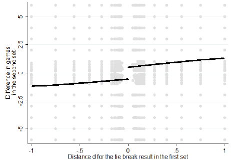
I’d display these data with a heat map rather than with overplotted points, but you get the idea.
This looked reasonable to me, but Guy Molyeneux sent in some skeptical comments, which I’ll give, followed by Page’s response. Molyeneux writes:
If I’ve followed the methodology correctly, I [Molyneaux] believe it’s wrong in critical respects. The biggest problem is that the regressions run on either side of the cutoff – an infinitely long tiebreaker — appear to be duplicative. One regression estimates that a player who loses set #1 will outscore his opponent by about .5 games in the second set. But he then also calculates the impact of losing the first set – .5 of course – and then adds them together to say a win is worth one full win. But the first regression already captured the impact of losing as well as the impact of winning, because the dependent variable is the second set differential between set #l’s winning and losing players. The result is a series of perfectly symmetrical but redundant graphs. And any variation from zero will necessarily create a “discontinuity” that is twice the real magnitude of the treatment effect.
Beyond that, it’s not clear that his device of looking only at long tiebreakers succeeds in creating a pool of contests between two equal players (such that we can infer any carryover from a first set victory is the result of that victory, not the player’s superior skill). In fact, the average difference in seeding between the winner and loser in long tiebreaks of 14 points or more (about 2 seeds) is the same as we see in 7-5 tiebreaks. And so is the disparity in second set games won. So it appears that the success of first set winners can be explained by their talent difference. (See Table 5).
Moreover, Page’s assumption that longer tiebreaks = more equal players is largely mistaken. Once a tiebreak has reached 6-6, its duration is largely a function of luck, not the players’ talent. The chance of each two-point segment ending in another tie is .558 if the players are evenly matched and win 67% of their serves, but is still .553 — essentially the same — if one player wins 62% and the other 72% of serves. A superior player is more likely to win a long tie break – the 72% service winner will win 61% of tiebreaks against a 62% opponent – but the disparity has little impact on the length of the tiebreak. And thus even in long tiebreaks, the winner will tend to be a better player.
None of this precludes the possibility that winning the first set has a real effect. Page provides some other evidence later in the paper that’s intriguing. For example, when players split the first two sets of a match, the player who won the second is more likely to win the third. But even here the evidence is far from conclusive. And he doesn’t really address the most plausible (to me) explanation for the patterns he sees, which is that the players are learning about their opponents strengths, weaknesses, and patterns of play over the course of the match, and one player is thus developing an advantage over his opponent which then continues in following sets.
Molyneaux’s key point seems to be that a tiebreaker, even if close, isn’t as random as it might seem. It’s an interesting example of a discontinuity analysis where the discreteness of the measure induces a gap near the discontinuity point. On the upside, Page’s sample size is large enough that it doesn’t seem like we’ll get tangled in the sorts of statistical-significance issues that made Berger and Pope’s basketball study so inconclusive.
I sent the above comments to Lionel Page, who responded as follows:
I [Page] thank Guy for reading my paper. I understand his first point, but it is just a definition issue. They are two ways to describe the effect and the one I used was the simplest given the technique I used. Fundamentally, I do not think that there is a “best definition”, it is simply important to bear in mind the two possible views. I wanted to make this point clearer in the paper, your comment definitively convince me to do it (thanks!).
I also understand perfectly your concern Guy on the second point but the paper went in great length to make this point quite solid empirically. The best way to answer this is to compare Figure 4 to Figure 6. If players winning tie break are simply better, they should win more in the first set when they win a close tie break in the second set AS they win more in the second set after winning a close tie break in the first set. The complete asymmetry between Figure 4 and 6 shows that the “effect” only exists in the direction of the arrow of time which is consistent with a “momentum” explanation and indicates that there is no reason to suspect that players winning a tie break are systematically better.
I did not answer the last point on the 1-1 situation for simplicity. The identification assumption is actually slightly more questionable here for reasons I stress in section 3 (just before section 4). However, the result stays exactly the same when I control for possible differences in seeding numbers. I cannot control for unobservable, but the fact that the coefficient does not drop when I control for seeding numbers give me some reasonable confidence in the validity of the result.
Here are Page’s responses in more detail:
I [Page] thank Guy Molyneux for his comments. Here are answers to the points he raised.
* “The biggest problem is that the regressions run on either side of the cutoff – an infinitely long tiebreaker — appear to be duplicative.”
I understand this concern, it is in some sense a natural one but I must stress that this is not a problem. My choice of presentation of the results stems naturally from the statistical strategy used in the paper. I compare the outcome of a player if he wins versus the counterfactual: his outcome if he does not win (therefore if he loses). So this difference is effectively in some sense duplicative, it is the margin of victory plus the margin of defeat. On small samples these two measures could differ but as I use a very large sample they are close to be identical (around .5) and therefore it may look as if the effect is wrongly double what it should be.
In fact to say that the “effect” is counted twice here, it is just to have another definition of the “effect” than in the paper. I define the effect as the effect of winning versus losing. One can decide that the effect is the difference in scores between the winner of the first
set and the loser: 0.5. But the gain in intuition here is lost in the definition of the effect: “winning versus …”? To sum up it is just that there are two ways to look at the effect, I stressed on the first one which stems from a standard statistical approach. The second way to define the effect is also present in Table 3. In any case, whatever the way you define the effect it is highly significant statistically and practically.* “Beyond that, it’s not clear that his device of looking only at long tiebreakers succeeds in creating a pool of contests between two equal players”
It is a natural concern. The paper goes in great length to carefully expose why we may confidently accept this assumption. Here is a summary of the arguments.
1) First, we may be confident in the hypothesis because there are no observable differences between players competing in tie breaks of 20 points or more.
a) There is no difference in seeding numbers between players playing long tie breaks. Guy quotes Table 5 as evidence of a difference in seeding numbers. Actually, on the contrary, for long tie breaks of more than 20 points there is no significant difference in seeding numbers (the difference is not “2” as Guy noted but “0.03” and it is nowhere near to be significant), while the difference in result in the second set is still highly significant (0.6 games at P<0.001). b) There is no difference in betting odds (winning odds) between players playing very long tie breaks (Table 5). Betting odds contain much more information than seeding numbers about the quality of players. These two facts are very important. If, as Guy suspects, players winning tie breaks are better, then we should see that they have a better ranking on average or that they have more chances to win the match ex-ante (measured by the betting odds). It is not the case, they have on average the same seeding numbers and the same betting odds. For this reason one may consider the assumption that these players are on average similar in ability very reasonable. However one may still wonder: "you show that they are equal on characteristics you observe, but they may still be differences regarding characteristics you do not observe". For instance the day of the match a player can be sick and this is neither captured by their seeding number nor by the betting odd. Due to this illness the player may not play as well, lose the tie break and lose the next set. So in some sense winning a tie break could just "reveal" some hidden difference in ability. For this reason the second point is certainly the most convincing answer to this concern. 2) Second, we may be confident in the hypothesis because there are no differences in unobservable characteristics between winners and losers of very long tie breaks. If a player winning a tie-break is on average playing better than his opponent then he should be better during ANY set of the match. A simple way to test that the "momentum" observed is not spurious (simply due to differences in players ability) is to check that while a momentum can be observed from one set to the next, there is no "backward momentum". In particular players winning a second set tie break should on average be better in the first set. If it was the case, it could not be due to the psychological effect of winning the second set and it would be the evidence that winners of tie break are simply better players. Figure 6, presents the result of this analysis (also called placebo regression). It is for me one of the most compelling results of the paper: players winning in the second set in a close tie break do not on average do better than their opponent in the first set. It is only when one looks at players winning a close tie break in the first set that one observes a difference in the second set. This is clearly an indication that one can accept the hypothesis that players opposed in close tie breaks have on average identical abilities.
It’s great to see this sort of dialogue. One thing I love about this discussion is the necessary interplay between statistical and substantive concerns, something that we see all the time in real examples but which rarely, rarely comes up in textbooks, which typically present a stark day-and-night distinction between correct and flawed analyses.
Lionel: Thanks for your thoughtful reply. Let me start by repeating that I am not arguing that there is no effect from winning a prior set. There may be. I'm simply questioning whether the evidence marshaled in the paper demonstrates such an effect. Let me respond to each of the 3 key issues.
1) On the question of whether the effect is .5 games or 1 game, perhaps this is a semantic difference. But you say that you want to "compare the outcome of a player if he wins versus the counterfactual: his outcome if he does not win (therefore if he loses)." Let us say the set 1 winner wins 5 games in set 2 (on average), while the loser wins 4.5 games. So if I win set 1, I will win .5 games more than if I were to lose, which I think most readers would consider the difference between winning and losing. Now, is it also true that my opponent will win .5 fewer games — but that must be true, as tennis is a zero sum game. Surely a reader of your paper could get the impression that the winner of a set can be expected to win one more game than his opponent in the next set — but that would be incorrect.
Suppose you did a similar analysis of years of education and annual income, with 12 years (HS diploma) as your cutoff. You find that those with 12 years education earn $5,000 more than those with 11.99 years. And you also find that those with 11.99 years earn $5,000 less than those with 12 years. Will you then report that a HS diploma increases income by $10,000?
More importantly, I'm puzzled by this statement: "On small samples these two measures could differ but as I use a very large sample they are close to be identical (around .5) and therefore it may look as if the effect is wrongly double what it should be." Is not your sample of long tiebreaks in which player A beats player B the same as the sample in which B beats A — except you reverse the letters? It seems to me the samples, even if small, must produce estimates that are identical on both sides. Perhaps I'm misunderstanding your method here….
* *
2) I remain unpersuaded that players in long tie breaks are effectively equal in ability for both theoretical and empirical reasons. You make a key assumption in the paper “It is natural to consider that the longer the tie break, the closer the results was. The longer the tie-break the more the players have shown closeness in ability in the game, since they were not able to distance each other earlier.” I agree that this seems “natural” (intuitive), but surprisingly it just isn’t the case. There should be very little difference in the talent spread between 8-6 tiebreaks and longer tie breaks. Once players reach 6-6, the probability of a long tie break depends very little on the relative talent of the players, and almost entirely on the proportion of service points players in general tend to win. Two players who each win 60% of their serves will reach another deuce 52.0% of the time; but if one player is 65% and the other 55% (a huge talent difference), you still get another deuce 51.5% of the time! And if you look at your data, you will see deuces are reached 52% of the time at 6-6, 54% at 7-7, and 52% at 8-8. If talent differences were narrowing at each stage and a narrow talent difference meant an increased chance of another deuce – as you believe – the deuce percentage should grow. But it does not.
Empirically, a look at the seeding data (table 5) shows that the first set winner is consistently about 2 seeds better than the loser in tiebreaks of 12, 14, 16, and 18 points – there is no pattern of narrowing talent spread. Only in your final cell of 20+ games does the difference in seeding disappear. Other than this one 20+ point cell, all the data suggests a constant talent advantage for the first set winner for tie breaks of 12 or more points. And this is critical, because there is of course no data at, or very close to, your cutoff. So your key finding really rests entirely on the 20+ sample of 1733 matches, not the 72,294 “close tie breaks” referenced in the abstract. Given that there is no theoretical reason for the talent spread to suddenly narrow at 20 points, I'm skeptical this tells us much. And I don’t consider the betting odds data compelling because of the very small and non-random samples (and this data indicates a constant talent disparity from 7-3 thru 9-7, at which point the sample becomes tiny).
(BTW, when I said that before that there is a 2-seed difference in “long tie breaks” I meant tie breaks of 14 games or more. You sometimes show these results, sometimes only 20+ points. I didn’t intend to misrepresent your findings.)
Also, if you are correct that the first set victory is worth .5 games, then your tie break results in table 5 imply that a 2-seed advantage is only worth about .15 additional games. Yet when we see a 4-seed spread (e.g. 7-5 games, or 7-1 tie break) that seems to convey about .6 wins – 4 times as much. Overall, the data in table 5 seems much more consistent with the idea that a 2-seed difference signifies a .5 games difference in ability, including in the 14+ point tie breaks.
Moreover, even equivalent seedings need not mean the true win% for both players in these matches is 50%. There is not a single generic “tennis skill” — players have specific strengths and weaknesses that match up well or not against an individual opponent, so it’s reasonable to assume that in any given pairing of closely-ranked players one of them would win 53% or 57% of an infinite # of sets. And the chance that the better player will win the tie break is virtually the same in a 14-point tiebreak or a 20-point tiebreak.
In short, we agree that there is little difference in 2nd set results from 12-point tie breaks on. To me, that simply suggests longer tie breaks fail to narrow the talent gap, which is consistent with what probability tells us about longer tie breaks.
* *
Third issue: on the other side, there is the evidence of no “backward momentum.” This is a strong argument. But I would find it much more persuasive if you provided a version of Table 5 for this data: how many of these close 2nd set tie breaks were there, what were the relative seedings and betting odds, etc. Perhaps Andrew could post that here if you provide it. Looking at figure 6, it looks to me like 2nd set tie break winners do in fact win more than 50% of the games in set 1. If so, the difference then is only in your projection of what theoretically happens in an infinite tie break, which again is sensitive to the results of fairly small samples of 20+ point tie breaks.
Moreover, theoretically it could be the case that better players win first set tie breaks, but not 2nd set tie breaks. Admittedly, that seems unlikely. But whatever may be true of 2nd set tie breaks, your case relies on the proposition that the players winning 1st set tie breaks are not better players than the losers. And the evidence for that claim I think is weak.
Again, I find it plausible that winners of one set are more likely to win the following set, controlling for talent. In fact, I'd be surprised if there were not any such effect, as I would expect that tennis players learn more about their opponents' strengths, weaknesses, and tactical choices over the course of a match, so that each successive set is a better measure (on average) of their true abilities against one another than are prior sets. (I'm assuming that many of these matches at the lower professional levels include players who have not played many prior matches against each other.) That would account for less "backward momentum." But that still would still leave this as an issue of talent (non-stable), rather than an effect of winning per se.
* *
Lastly, a couple of stray thoughts/questions for you:
*If the winner effect is real, this should have consequences for the distribution of wins in 5-set matches. I would think that ABABA outcomes would be quite rare, as they require 4 reversals of momentum, while AABBB and AABBA are much more common. Is that in fact true?
*You find a similar advantage for 2nd set winners in a 1-1 match. However, players who win the 2nd set despite the opponent’s momentum must be, on average, better players than their opponent. So shouldn’t second set winners enjoy a 3rd set margin considerably larger than .5 games?
Guy, here are quick answers
1) The example you give on the effect of a diploma does not present the same situation than in the paper. The treatment is having versus not having a diploma, so the difference must be counted once only. Here the difference is winning versus losing.
I do not duplicate the sample. Matches on both sides of Figure 4 and 6 are different matches, I have just randomly allocated them to make sure there is no selection bias. If I was using the matches twice I would artificially increase the power of the statistical test. As the matches are different, the effects measured on both sides can differ on small samples.
2) & 3) It is not a problem if some tie breaks present differences in players ability. I should even say something more subtle: the identification hypothesis would still be acceptable even if there were differences for all the categories of Table 5, even if players winning versus losing tie breaks of more than 20 points were not identical. What is important is that, at the limit, when the tie breaks tend toward infinity, the players tend to be identical. The effect must be estimated in d=0 (for infinite tie-break). This is the principle of the discontinuity design. The calculation of an optimal bandwidth ensures that the local information given by the long tie breaks is used optimally to estimate the effect at the threshold by local linear regression.
The evidence in the paper is quite compelling regarding the fact that players have similar ability in very close tie breaks. You are concerned by the fact that this is only the case for tie breaks over 20 points, but it is exactly the point of the estimation. There are more than 1,200 of such tie breaks in the data which is enough to make sure that this non significance is not a statistical aberration. In any case, even if you were not to believe in this fact, you may admit that asymptotically it is the case for infinite tie breaks and that is where the effect is estimated.
For this reason, the comparison of Figure 4 and 6 is telling: there is no difference in d=0 for Figure 6 while there is an important one in Figure 4.
Regarding your last two points.
* The paper discusses two different notions of momentum. Each of them would have different types of effects. In the case of a state dependency, the effect is not clear (it would most likely depends on additional hypotheses in the model). In any case, a simple observation of the sequence is most likely to be unconclusive as lots of things happen in a match for which we cannot control for. It is why the discontinuity design is useful here, it can however only be used in limited situations.
* I discuss this point at the end of Section 3. Due to the idea you raise, the identification is not as clear cut. However, the result stays exactly the same when I control for seeding numbers which is quite reassuring about the validity of the result.
off-topic
Dear professor Gelman,
I don't know if you are aware of a discussion in polmeth list about reporting p-values instead of graphics in political science journals. Since this is a topic you are always discussing in your Blog, I though it would be nice to know your opinion about this little controversy.
Below I quote one of the e-mails…
"Well, tastes differ. I, for one, don't think it is so obvious that graphs are underutilized and tables overutilized in political science
journals. Obviously, it is often most helpful to have both. As electronic publishing becomes the norm, that will presumably become increasingly common. In the meantime, however, when space constraints necessitate a choice my preference will usually be for the table. Not
always, of course — a scatterplot with lowess regression superimposed has no satisfactory tabular equivalent. But if the point is simply to report regression coefficients, graphs are likely to take more space and convey the relevant information much less precisely. For making a point in an undergraduate textbook or an op-ed piece that may be fine, but for
a scholarly journal article accuracy and efficiency should often take precedence over "present[ing] your work in the most compelling visual manner," as Mike puts it.
Having said that, it should be obvious where I stand on Anthony's original question about reporting point estimates. Yes, by all means —
but with the associated standard errors as well, so that readers can appropriately gauge the relevant uncertainty. (Do most readers "really
understand" what these mean? That, too, is largely a matter of context. For an undergraduate textbook, probably not. For a scientific journal, I'd hope so.) Simply reporting p-values will only be informative to
readers who happen to be interested in the null hypothesis that the relevant parameter value is zero, which I almost never am. The point of
doing _quantitative_ analysis, as I see it, is to learn something about the _magnitudes_ of empirical relationships, and that is what the point estimates (and standard errors) convey.
Larry"
Best Regards
Manoel Galdino
phdd student of Political Science, Brasil.
Hello Professor Gelman,
This is the first post I read of yours and will more than likely go through the rest of your sports post. One thing is for sure, you engaged me (and probably many other students) by co-mingling sports and statistics.
I played tennis growing up as a kid and just from experience can confirm the 1st set statistic. As in most sports, it's all about momentum.
You need to take the knowledge you have and participate in betting.
Good luck!
Fascinating discussion. I found your page doing a google search on 'momentum effect and tennis' since I've been observing and collecting data for something similar. I wanted to see if there were any papers written on the subject and happy to see the discussion is alive and well. My observation has to do with the effect that winning the first point of every game has on the outcome of the game. I'm not a statistician but I recruited a friend and Prof. of Statistics at UCLA to look at some of my data. Some very interesting results. Of course, they lack the scientific rigor necessary to make a solid argument, but if interested I urge you to pay attention to the upcoming Wimbledon. You may be quite surprised. In essence, if the receiver wins the first point of a game s/he has a greater chance of breaking than would be expected. Thanks, and continue the discussion. Fascinating stuff.
Roberto Donati MA MFT – Los Angeles