A Bayesian posterior distribution of a parameter demonstrates the uncertainty that arises from being a priori uncertain about the parameter values. But in a classical setting, we can obtain a similar distribution of parameter estimates through the uncertainty in the choice of the sample. In particular, using methods such as bootstrap, cross-validation and data splitting, we can perform the simulation. It is then interesting to compare the Bayesian posteriors with these. Finally, we can also compare the classical asymptotic distributions of parameters (or functionals of these parameters) with all of these.
Let us assume the following contingency table from 1991 GSS:
| Belief in Afterlife | ||
| Gender | Yes | No/Undecided |
| Females | 435 | 147 |
| Males | 375 | 134 |
We can summarize the dependence between gender and belief with an odds ratio. In this case, the odds ratio is simply θ= (435*134)/(147*375)=1.057 – very close to independence. It is usually preferable to work with the natural logarithm of the odds ratio, as its “distribution” is less skewed. Let us now examine the different distributions of log odds ratio (logOR) for this case, using bootstrap, cross-validation, Bayesian statistics and asymptotics.
Asymptotics
The large-sample approximating normal distribution has the mean of log θ, and a particular standard deviation, but the expression is nasty to typeset in HTML.
Bayesian
We have to assume a model. We will simply model the data as arising from a multinomial, using the usual symmetric Dirichlet prior with α=1. The odds ratio is then computed using the probabilities in the posterior, not using the counts.
Bootstrap
logOR is computed as above from the sample but from bootstrap resamples (samples of equal size from the original sample but with replacement).
K-fold Cross-Validation
The data is divided into K groups of approx. equal size, and K “versions” of the logOR are computed by omitting one of the groups and then estimating from the sample.
9:1 Data Splitting
logOR is computed from a random selections (without replacement) of 90% of the data.
Results
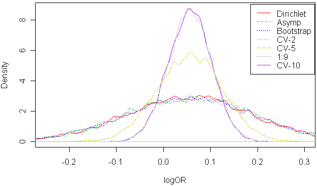
10000 samples of logOR were drawn using the above methodologies. We can see that bootstrap, Bayes, asymptotics and 2-fold cross-validation yield very similar distributions of logOR. On the other hand, k-fold cross-validation results in distinctly different distributions. Leave-one-out is not even shown.
Conclusion
Different assumptions lead to different conclusions. And the choice of splitting/cross-validation/bootstrap/asymptotics is the same kind of a prior assumption as is the Bayesian prior. Which assumption is correct? ;) Which assumption is easier to explain? What do assumptions mean?
While 1091 cases are quite a few, if the above experiment was repeated with a much smaller number of cases, the Bayesian approach would start making more sense than others. But when the number of cases is large, there is no major difference.