Seth Roberts

I met Seth back in the early 1990s when we were both professors at the University of California. He sometimes came to the statistics department seminar and we got to talking about various things; in particular we shared an interest in statistical graphics. Much of my work in this direction eventually went toward the use of graphical displays to understand fitted models. Seth went in another direction and got interested in the role of exploratory data analysis in science, the idea that we could use graphs not just to test or even understand a model but also as the source of new hypotheses. We continued to discuss these issues over the years; see here, for example.

At some point when we were at Berkeley the administration was encouraging the faculty to teach freshman seminars, and I had the idea of teaching a course on left-handedness. I’d just read the book by Stanley Coren and thought it would be fun to go through it with a class, chapter by chapter. But my knowledge of psychology was minimal so I contacted the one person I knew in the psychology department and asked him if he had any suggestions of someone who’d like to teach the course with me. Seth responded that he’d be interested in doing it himself, and we did it.

After we taught the class together we got together regularly for lunch and Seth told me about his efforts in self-experimentation involving sleeping hours and mood. One of his ideas was to look at large faces in the morning (he used tapes of late-night comedy monologues). This all seemed a bit sad to me, as Seth lived alone and thus did not have anyone to talk with in the morning directly. On the other hand, even those of us who live in large families do not always spend the time to sit down and talk over the breakfast table.

Seth’s self-experimentation went slowly, with lots of dead-ends and restarts, which makes sense given the difficulty of his projects. I was always impressed by Seth’s dedication in this, putting in the effort day after day for years. Or maybe it did not represent a huge amount of labor for him, perhaps it was something like a diary or blog which is pleasurable to create, even if it seems from the outside to be a lot of work. In any case, from my perspective, the sustained focus was impressive.

Seth’s academic career was unusual. He shot through college and graduate school to a tenure-track job at a top university, then continued to do publication-quality research for several years until receiving tenure. At that point he was not a superstar but I think he was still considered a respected member of the mainstream academic community. But during the years that followed, Seth lost interest in that thread of research (you can see this by looking at the dates of most of his highly-cited papers). He told me once that his shift was motivated by teaching introductory undergraduate psychology: the students, he said, were interested in things that would affect their lives, and, compared to that, the kind of research that leads to a productive academic career did not seem so appealing.

I suppose that Seth could’ve tried to do research in clinical psychology (Berkeley’s department actually has a strong clinical program) but instead he moved in a different direction and tried different things to improve his sleep and then, later, his skin, his mood, and his diet. In this work, Seth applied what he later called his “insider/outsider perspective”: he was an insider in that he applied what he’d learned from years of research on animal behavior, an outsider in that he was not working within the existing paradigm of research in physiology and nutrition.

At the same time he was working on a book project, which I believe started as a new introductory psychology course focused on science and self-improvement but ultimately morphed into a trade book on ways in which our adaptations to Stone Age life were not serving us well in the modern era. I liked the book but I don’t think he found a publisher. In the years since, this general concept has been widely advanced and many books have been published on the topic.

When Seth came up with the connection between morning faces and depression, this seemed potentially hugely important. Were the faces were really doing anything? I have no idea. On one hand, Seth was measuring his own happiness and doing his own treatments on his own hypothesis so the potential for expectation effects are huge. On the other hand, he said the effect he discovered was a surprise to him and he also reported that the treatment worked with others. Neither he nor, as far as I know, anyone else, has attempted a controlled trial of this idea.

Seth’s next success was losing 40 pounds on his unusual diet, in which you can eat whatever you want as long as each day you drink a cup of unflavored sugar water, at least an hour before or after a meal. To be more precise, it’s not that you can eat whatever you want—obviously, if you live a sedentary lifestyle and you eat a bunch of big macs and an extra-large coke each day, you’ll get fat. The way he theorized that his diet worked (for him, and for the many people who wrote in to him, thanking him for changing their lives) was that the carefully-timed sugar water had the effect of reducing the association between calories and flavor, thus lowering your weight set-point and making you uninterested in eating lots of food. I asked Seth once if he thought I’d lose weight if I were to try his diet in a passive way, drinking the sugar water at the recommended time but not actively trying to reduce my caloric intake. He said he supposed not, that the diet would make it easier to lose weight but you’d probably still have to consciously eat less.

In his self-experimentation, Seth lived the contradiction between the two tenets of evidence-based medicine:
1. Try everything, measure everything, record everything.
2. Make general recommendations based on statistical evidence rather than anecdotes.
Seth’s ideas were extremely evidence-based in that they were based on data that he gathered himself or that people personally sent in to him, and he did use the statistical evidence of his self-measurements, but he did not put in much effort to reduce, control, or adjust for biases in his measurements, nor did he systematically gather data on multiple people.

I described Seth’s diet to one of my psychologist colleagues at Columbia and asked what he thought of it. My colleague said he thought it was ridiculous. And, as with the depression treatment, Seth never had an interest in running a controlled trial, even for the purpose of convincing the skeptics. Seth and I ended up discussing this and related issues in an article for Chance, the same statistics magazine where in 2001 Seth had published his first article on self-experimentation.

Seth’s breakout success happened gradually, starting with a 2005 article on self-experimentation in Behavioral and Brain Sciences, a journal that publishes long articles followed by short discussions from many experts. Some of his findings from the ten of his experiments discussed in the article:

Seeing faces in the morning on television decreased mood in the evening and improved mood the next day . . . Standing 8 hours per day reduced early awakening and made sleep more restorative . . . Drinking unflavored fructose water caused a large weight loss that has lasted more than 1 year . . .

As Seth described it, self-experimentation generates new hypotheses and is also an inexpensive way to test and modify them. One of the commenters, Sigrid Glenn, pointed out that this is particularly true with long-term series of measurements that it might be difficult to do on experimental volunteers.

About half of the published commenters loved Seth’s paper and about half hated it. The article does not seem to have had a huge effect within research psychology (Google Scholar gives it 30 cites) but two of its contributions—the idea of systematic self-experimentation and the weight-loss method—have spread throughout the popular culture in various ways. Seth’s work was featured in a series of increasingly prominent blogs, which led to a newspaper article by the authors of Freakonomics and ultimately a successful diet book (not enough to make Seth rich, I think, but Seth had simple tastes and no desire to be rich, as far as I know). Meanwhile, Seth started a blog of his own which led to a message board for his diet that he told me had thousands of participants.

On his blog and elsewhere Seth reported success with various self-experiments, most recently a claim of improved brain function after eating half a stick of butter a day. I’m skeptical, partly because of his increasing rate of claimed successes. It took Seth close to 10 years of sustained experimentation to fix his sleep problems, but in recent years it seemed that all sorts of different things he tried were effective. His apparent success rate was implausibly high. What was going on? One problem is that sleep hours and weight can be measured fairly objectively, whereas if you measure brain function by giving yourself little quizzes, it doesn’t seem hard at all for a bit of unconscious bias to drive all your results. I also wonder if Seth’s blog audience was a problem: if you have people cheering on your every move, it can be that much easier to fool yourself.

Seth had a lot of problems with academia and a lot of legitimate gripes. He was concerned about fraud (and the way that established researchers often would rather cover up an ethical violation than expose it) and also about run-of-the-mill shabby research, the sort of random and unimportant non-findings that fill up our scientific journals. But Seth’s disconnect from the academic research world was unfortunate, for two reasons. First, others were not getting the advantages of his perspective; second, he was not engaging with the sort of serious criticism that can make one’s work better. I certainly don’t think an academic connection is necessary for someone to engage with criticism, but it provides many opportunities, for those of us lucky enough to be so situated.

Seth was a complete outsider in the psychology department at Berkeley for decades and eventually took early retirement while barely in his fifties. I was surprised: as I told Seth, being a university professor is such a cushy job, they pay you and you don’t have to do anything. He responded dryly that retirement works the same way. As things turned out, though, he did take a new job, teaching at a university in China. That worked out for him, partly because he enjoyed undergraduate teaching—as he put it, the key is to work with the students’ unique strengths, rather than to spend your time trying to mold the students into miniature versions of yourself.

In the late 1990s, my friend Rajeev and I would sometimes go to poetry slams. Our most successful effort was once when I read Rajeev’s poem aloud and he read mine. It turns out that it’s easier to be expressive with somebody else’s words. Another thing I learned at that time was that people have a lot of problem pronouncing “Rajeev.” It’s pronounced just as it’s spelled, but people kept trying to say something like “Raheev” but in a hesitant voice as if it was this super-unusual name.

Anyway, one I idea I had, but which I never carried out, was to write down a bunch of facts about Seth and read them off, one at a time, completely deadpan. The gimmick would be that I’d come up on the stage, pull out a deck of index cards and ask a volunteer in the front row to shuffle them. I’d then read them off in whatever order they came up. The idea was that Seth was such an unusual person that his facts would be interesting however they came out.

In order to preserve some anonymity, my plan was to refer to Seth as “Josh.” (I think of “Josh” as an equivalent name to Seth, just as “Samir” is an alternative-world name for Rajeev.) I’m not sure what happened to my list of Josh sentences—I never actually put them into an act—but here a few:

Josh rents rats.

Josh stares at Jay Leno in the morning.

Josh works on a treadmill.

Josh lives in the basement.

There are a bunch more that I just can’t remember. Seth used to stay with me when he’d visit NY (I moved to Columbia because my Berkeley colleagues didn’t want me around; Seth and I joked that we should trade jobs because he liked NY but Columbia would never hire him), but it’s been several years since we’ve hung out and it’s hard for me to remember some of the unusual things he’d do. OK, I do remember one thing: he would often strike up conversations with perfect strangers, for example asking someone at the next table at a restaurant what they were eating or asking someone on the subway what they were reading. Most of the time this didn’t bother me—actually, I found it interesting, as I could get some information without suffering the difficulty of talking with a stranger. One time, though, he blocked me: I don’t think he realized what was going on at the time, but I was chatting up someone at some event—I can’t recall any of the details here (it was something like 15 years ago) but I do remember that he joined in the conversation and started yakking his head off until she drifted away with no chance that I could see for recovery on my part. Afterward, I berated Seth: What were you thinking? You ruined my chances with her, etc. . . . but he’d just been oblivious, just starting one more conversation with a stranger. Seth was always interested in what people had to say. His conversational style was to ask question after question after question after question. This didn’t really show up in his online persona. It’s interesting how our patterns of writing can differ from how we speak, and how our interactions from a distance can differ from our face-to-face contacts.

One of Seth’s and my shared interests was Spy magazine, that classic artifact of the late 1980s. When I found out that Seth had actually written for Spy, I was so impressed!

Here was our last contact, which won’t be of interest to anyone except to me because it happened to be the last time I heard from him:

Screen Shot 2014-04-29 at 10.39.08 PM

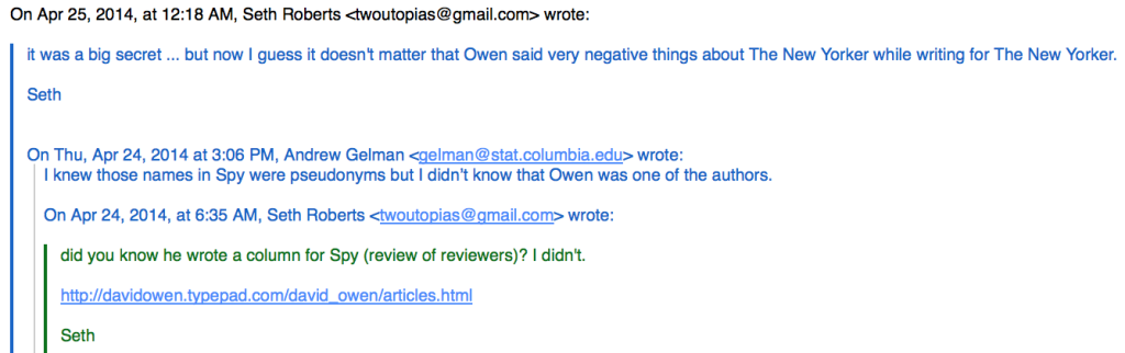
My friend is gone. I miss him.

Ken Rice presents a unifying approach to statistical inference and hypothesis testing

Ken Rice writes:

In the recent discussion on stopping rules I saw a comment that I wanted to chip in on, but thought it might get a bit lost, in the already long thread. Apologies in advance if I misinterpreted what you wrote, or am trying to tell you things you already know.

The comment was: “In Bayesian decision making, there is a utility function and you choose the decision with highest expected utility. Making a decision based on statistical significance does not correspond to any utility function.”

… which immediately suggests this little 2010 paper; A Decision-Theoretic Formulation of Fisher’s Approach to Testing, The American Statistician, 64(4) 345-349. It contains utilities that lead to decisions that very closely mimic classical Wald tests, and provides a rationale for why this utility is not totally unconnected from how some scientists think. Some (old) slides discussing it are here.

A few notes, on things not in the paper:

* I know you don’t like squared-error loss on its own – and I think this is fair – but (based on prior work by others) it’s highly plausible the paper’s specific result extends to give something very similar for whole classes of bowl-shaped loss functions – that describe much the same utility in a less mathematically-tractable way. Also, I’m not claiming the utilities given are the *only* way to interpret such decisions.

* Even if one doesn’t like either squared-error loss or its close relatives, the framework at least provides a way of saying what classical tests and p-values might mean, in the Bayesian paradigm. That they mean something rather different to Bayes factors & posterior probabilities of the null is surprising to many people, particularly those keen to dismiss all use of p-values. I really wrote the paper because I was fed up with unrealistic point-mass priors being the only Bayesian way to get tests; like you, I work in areas where exactly null associations are really hard to defend. [Yup—ed.]

Here’s the abstract of Rice’s 2010 paper:

In Fisher’s interpretation of statistical testing, a test is seen as a ‘screening’ procedure; one either reports some scientific findings, or alternatively gives no firm conclusions. These choices differ fundamentally from hypothesis testing, in the style of Neyman and Pearson, which do not consider a non-committal response; tests are developed as choices between two complimentary hypotheses, typically labeled ‘null’ and ‘alternative’. The same choices are presented in typical Bayesian tests, where Bayes Factors are used to judge the relative support for a null or alternative model. In this paper, we use decision theory to show that Bayesian tests can also describe Fisher-style ‘screening’ procedures, and that such approaches lead directly to Bayesian analogs of the Wald test and two-sided p-value, and to Bayesian tests with frequentist properties that can be determined easily and accurately. In contrast to hypothesis testing, these ‘screening’ decisions do not exhibit the Lindley/Jeffreys paradox, that divides frequentists and Bayesians.

This could represent an important way to look at statistical decision making.

Bayesian Uncertainty Quantification for Differential Equations!

Screen Shot 2014-04-29 at 7.37.02 AM

Mark Girolami points us to this paper and software (with Oksana Chkrebtii, David Campbell, and Ben Calderhead). They write:

We develop a general methodology for the probabilistic integration of differential equations via model based updating of a joint prior measure on the space of functions and their temporal and spatial derivatives. This results in a posterior measure over functions reflecting how well they satisfy the system of differential equations and corresponding initial and boundary values. We show how this posterior measure can be naturally incorporated within the Kennedy and O’Hagan framework for uncertainty quantification and provides a fully Bayesian approach to model calibration. . . . A broad variety of examples are provided to illustrate the potential of this framework for characterising discretization uncertainty, including initial value, delay, and boundary value differential equations, as well as partial differential equations. We also demonstrate our methodology on a large scale system, by modeling discretization uncertainty in the solution of the Navier-Stokes equations of fluid flow, reduced to over 16,000 coupled and stiff ordinary differential equations.

This looks interesting and potentially very important. In the world of applied math, the problem is sometimes called “uncertainty quantification” or UQ; in statistics we call it Bayesian inference. In any case it can be difficult because for big problems these differential equations can take a long time to (numerically) solve. So there would be a lot of use for a method that could take random samples from the posterior distribution, to quantify uncertainty without requiring too many applications of the differential equation solver.

One challenge is that when you run a differential equation solver, you choose a level of discretization. Too fine a discretization and it runs too slow; too coarse and you’re not actually evaluating the model you’re interested in. I’ve only looked quickly at this new paper of Chkrebtii et al., but it appears that they are explicitly modeling this discretization error rather than following the usual strategy of applying a very fine grid and then assuming the error is zero. The idea, I assume, is that if you model the error you can use a much coarser grid and still get good results. This seems possible given that do apply any of these methods you need to apply the solver many many times.

As the above image from their paper illustrates, each iteration of the algorithm proceeds by running a stochastic version of the differential-equation solver. As they emphasize, they do not simply repeatedly run the solver as is; rather they go inside the solver and make it stochastic as a way to introduce uncertainty into each step. I haven’t read through the paper more than this but it looks very interesting and it feels right in the sense that they’ve added some items to the procedure so it’s not like they’re trying to get something for nothing.

Also, movies:

Crowdstorming a dataset

Raphael Silberzahn writes:

Brian Nosek, Eric Luis Uhlmann, Dan Martin, and I just launched a project through the Open Science Center we think you’ll find interesting.

The basic idea is to “Crowdstorm a Dataset”. Multiple independent analysts are recruited to test the same hypothesis on the same data set in whatever manner they see as best. If everyone comes up with the same results, then scientists can speak with one voice. If not, the subjectivity and conditionality of results on analysis strategy is made transparent. For this first project, we are crowdstorming the question of whether soccer referees are more likely to give red cards to dark skin toned players than light skin toned players.

The full project description is here.

If you’re interested in being one of the crowdstormer analysts, you can register here.

All analysts will receive an author credit on the final paper. We would love to have Bayesian analysts represented in the group. Also, please feel free to let others know about the opportunity, anyone interested is welcome to take part.

I have no idea how this will work out but it seems to be worth a try.

On deck this week

Mon: Crowdstorming a dataset

Tues: Ken Rice presents a unifying approach to statistical inference and hypothesis testing

Wed: The health policy innovation center: how best to move from pilot studies to large-scale practice?

Thurs: Heller, Heller, and Gorfine on univariate and multivariate information measures

Fri: Discovering general multidimensional associations

Sat: “The graph clearly shows that mammography adds virtually nothing to survival and if anything, decreases survival (and increases cost and provides unnecessary treatment)”

Sun: Honored oldsters write about statistics

White stripes and dead armadillos

Paul Alper writes:

For years I [Alper] have been obsessed by the color of the line which divides oncoming (i.e., opposing) traffic because I was firmly convinced that the color of the center line changed during my lifetime. Yet, I never could find anyone who had the same remembrance (or interest in the topic). The other day I found this this explanation that vindicates my recollection (and I was continuously out of the U.S. from 1969 to 1973):

The question of which color to use for highway center lines in the United States enjoyed considerable debate and changing standards over a period of several decades. By November 1954, 47 states had adopted white as their standard color for highway centerlines, with Oregon being the last holdout to use yellow. In 1958, the U.S. Bureau of Public Roads adopted white as the standard color for the new interstate highway system. The 1971 edition of the Manual on Uniform Traffic Control Devices, however, mandated yellow as the standard color of center lines nationwide. The changeover to the 1971 MUTCD standards took place between 1971 and 1975, with most done by the end of 1973, so for two years drivers still had to use the old and new. Yellow was adopted because it was already the standard color of warning signs, and because it was easy to teach drivers to associate yellow lines with dividing opposing traffic and white lines with dividing traffic in the same direction. . . .

Most European countries reserve white for routine lane markings of any kind. Yellow is used to mark forbidden parking, such as on bus stops.

Most countries in North and South America have yellow lines separating traffic directions. However, for example Chile has white such lines.

Armed with this knowledge, I have haphazardly been asking (annoying) American friends and relations as to what color they think the center line is now, let alone what it used to be. Young people get it right I guess because that is part of driver ed which they have recently completed; older people who drive a lot still claim the center line is white and always has been.

Wow! How could they think such a thing???

Alper continues:

If in fact so many Americans do not recall such an everyday occurrence what does this say about self-reporting and eye-witness testimony—like the famous gorillas across the screen in that classic psych study?

So, as a simple experiment is there a way of improving my haphazard sampling to give some statistical “oomph” to the contention that (older?) people are inattentive to their motoring surroundings to a remarkable degree? Redo the gorilla example by changing the color of the center line every few seconds while focusing attention on other aspects of driving? Does inattentiveness to color of the dividing line correlate with age, gender, handedness, SAT math score, religion, Vitamin D consumption, etc.?

Hmmm, could be interesting. Here’s my advice to any researchers out there who want to try this experiment. If you want to maximize your chances of getting it into Psychological Science, do several experiments, each with a nice small sample size—25 or 50 in each case should do it—and keep all your data-analysis options open.

Sleazy sock puppet can’t stop spamming our discussion of compressed sensing and promoting the work of Xiteng Liu

Some asshole who has a bug up his ass about compressed sensing is spamming our comments with a bunch of sock puppets. All from the same IP address: “George Stoneriver,” Scott Wolfe,” and just plain “Paul,” all saying pretty much the same thing in the same sort of broken English (except for Paul, whose post was too short to do a dialect analysis). “Scott Wolfe” is a generic sort of name, but a quick google search reveals nothing related to this topic. “George Stoneriver” seems to have no internet presence at all (besides the comments at this blog). As for “Paul,” I don’t know, maybe the spammer was too lazy to invent a last name?

Our spammer spends about half his time slamming the field of compressed sensing and the other half pumping up the work of someone named Xiteng Liu. There’s no excuse for this behavior. It’s horrible, a true abuse of our scholarly community.

If Scott Adams wants to use a sock puppet, fine, the guy’s an artist and we should cut him some slack. If that’s what it takes for him to get his creative juices flowing, I’ll accept it. But to use sock puppets to try to trash legitimate scientific work, that’s not cool.

I can only assume that Xiteng Liu would not appreciate that someone is spamming websites on his behalf. It’s not good for someone’s reputation to be associated with a sock puppet. I know that if someone were spamming on behalf of my research, I’d be really annoyed.

P.S. I realized I used “ass” twice in my first sentence above. That’s bad writing. Feel free to switch in some other expletive to make the sentence flow better.

P.P.S. Further discussion here from Igor Carron.

Revised statistical standards for evidence (comments to Val Johnson’s comments on our comments on Val’s comments on p-values)

As regular readers of this blog are aware, a few months ago Val Johnson published an article, “Revised standards for statistical evidence,” making a Bayesian argument that researchers and journals should use a p=0.005 publication threshold rather than the usual p=0.05.

Christian Robert and I were unconvinced by Val’s reasoning and wrote a response, “Revised evidence for statistical standards,” in which we wrote:

Johnson’s minimax prior is not intended to correspond to any distribution of effect sizes; rather, it represents a worst case scenario under some mathematical assumptions. Minimax and tradeoffs do well together, and it is hard for us to see how any worst case procedure can supply much guidance on how to balance between two different losses. . . .

We would argue that the appropriate significance level depends on the scenario and that what worked well for agricultural experiments in the 1920s might not be so appropriate for many applications in modern biosciences . . .

PNAS also published comments from Jean Gaudart, Laetitia Huiart, Paul Milligan, Rodolphe Thiebaut, and Roch Giorgi (“Reproducibility issues in science, is P value really the only answer?“) and Luis Pericchi, Carlos Pereira, and María-Eglée Pérez (“Adaptive revised standards for statistical evidence“), along with Johnson’s reply to all of us.

Val Johnson and I agree

Before getting to my disagreements with what Val wrote, I’d like to emphasize the important area where we agree. We both feel strongly dissatisfied with the existing default approach of scientific publication in which (a) statistical significance at the p=0.05 level is required for publication, and (b) results which are published and achieve p=0.05 are considered to be correct.

Val’s approach is to apply a minimax argument leading to a more stringent p-value threshold, whereas I’d be more interested in not using p-values (or related quantities such as Bayes factors) as publication thresholds at all. But we agree that the current system is broken. And I think we also agree that thresholds for evidence should depend on scientific context. For example, Val proposes a general cutoff of p=0.005 but he also writes approvingly (I think) that “P value thresholds of 3 × 10⁻⁷ are now standard in particle physics.” Again, I don’t like using any p-value threshold but I agree with Val that the current p=0.05 thing is causing problems. (Indeed, in some settings, I think it’s fine to report evidence that does not even reach the 0.05 level, if the problem is important enough. We discussed this in the context of the flawed paper on the effects of coal heating in China, where I argued that (a) their claim of p=0.05 statistical significance was a joke, but (b) maybe their claims should still be published, despite their inconclusive nature, because of the importance of the topic).

In short, Val and I agree with the Bayesian arguments made by Berger and others that p=0.05 provides weaker evidence that is typically believed. Where we disagree is in what to do about this.

Val Johnson and I disagree

In his reply to Christian and me, Val writes:

Gelman and Robert’s letter characterizes subjective Bayesian objections to the use of more stringent statistical standards, arguing that significance levels and evidence thresholds should be based on “costs, benefits, and probabilities of all outcomes.” In principle, this is a wonderful goal, but in practice, it is impossible to achieve. In most hypothesis tests, unique and well-defined loss functions and prior densities do not exist. Instead, a plethora of vaguely defined loss functions and prior densities exist. . . . Thousands of scientific manuscripts are written each year, and eliciting these distinct loss functions and priors on a case-by-case basis, and determining how to combine them, is simply not feasible. . . .

Just to be clear here: Christian and I nowhere used the term “subjective” in our letter, and indeed I do not consider our reference to decision analysis to be subjective, at least not any more subjective than the choice of a probability of 1/20 that drives Val’s calculations. The 1/20 level is objective only in the sociological sense that it represents a scientific tradition.

Val’s second point is that well-defined loss functions are difficult to achieve. I agree, and indeed in my own work I have rarely worked with formal loss functions or performed formal decision analyses. I am happy to report posterior inferences along with the models on which they are based. But Val is wanting to do more than this. He is trying to set a universal threshold for statistical significance. I don’t think this makes sense for the reasons Christian and I discussed in our letter. Finally, Val writes of the difficulty of eliciting loss functions and priors for the “thousands of scientific manuscripts [that] are written each year.” Sure, but one could make the same argument regarding other aspects of a scientific experiment, such as the design of the experiment, rules for data exclusion and data analysis, and choice of what information to include in the analyses. In some settings, it will be difficult to elicit a data model too, but the statistical profession seems to have no problem requiring researchers to do it.

Val also replies to one of our specific comments in this way:

The characterization of uniformly most powerful Bayesian tests (UMPBTs) as minimax procedures is inaccurate. Minimax procedures are defined by minimizing the maximum loss that a decision maker can suffer. In contrast, UMPBTs are defined to maximize the probability that the Bayes factor in favor of the alternative hypothesis exceeds a specified threshold.

I don’t really understand what Val is saying here, but I will accept that the term “minimax” has a technical meaning which does not correspond to his procedure. In any case, I stand by what Christian and I wrote earlier (setting aside the particular word “minimax”) that we can’t see it making sense to work with a worst-case probability that, in this case, does not correspond to any sensible prior distribution.

In short, I respect that Val is working on an important problem, but (a) I don’t really think we can do anything with the numbers that come out of his worst-case approach, and (b) I don’t like the general approach of seeking a universal p-value threshold.

An open site for researchers to post and share papers

Alexander Grossman writes:

We have launched a beta version of ScienceOpen in December at the occasion of the MRS Fall meeting in Boston. The participants of that conference, most of them were active researchers in physics, chemistry, and materials science, provided us with a very positive feedback. In particular they emphazised that it appears to be a good idea to offer scientists a free platform to collaborate with each other and to share draft versions of their next paper privately.

Meanwhile more than 1 million open access papers in the area of the natural sciences and medicine can be accessed via ScienceOpen, read, and commented or evaluated after publication. We call this concept post-publication peer review.

I don’t know anything about this but I thought I’d share it with you. I know a lot of people use Arxiv but that has some problems, maybe this will have some advantages.
Continue reading

Thinking of doing a list experiment? Here’s a list of reasons why you should think again

Someone wrote in:

We are about to conduct a voting list experiment. We came across your comment recommending that each item be removed from the list. Would greatly appreciate it if you take a few minutes to spell out your recommendation in a little more detail. In particular: (a) Why are you “uneasy” about list experiments? What would strengthen your confidence in list experiments? (b) What do you mean by “each item be removed”? As you know, there are several non-sensitive items and one sensitive item in a list experiment. Do you mean that the non-sensitive items should be removed one-by-one for the control group or are you suggesting a multiple arm design in which each arm of the experiment has one non-sensitive item removed. What would be achieved by this design?

I replied: I’ve always been a bit skeptical about list experiments, partly because I worry that the absolute number of items on the list could itself affect the response. For example, someone might not want to check off 6 items out of 6 but would have no problem checking off 6 items out of 10: even if 4 items on that latter list were complete crap, their presence on the list might make the original 6 items look better by comparison. So this has made me think that a list experiment should really have some sort of active control. But the problem with the active control is that then any effects will be smaller. Then that made me think that one might be interested in interactions, that is, which groups of people would be triggered by different items on the list. But that’s another level of difficulty…

And then I remembered that I’ve never actually done such an experiment! So I thought I’d bring in some experts. Here’s what they said:

Macartan Humphreys:

I have had mixed experiences with list experiments.

Enumerators are sometimes confused by them and so are subjects and sometimes we have found enumerators implementing them badly, eg sometimes getting the subjects to count out as they go along reading the list that kind of thing. Great enumerators shouldn’t have this problem, but some of ours have.

In one implementation that we thought went quite well we cleverly did two list experiments with the same sensitive item and different nonsensitive items, but got very different results. So that is not encouraging.

The length of list issue I think is not the biggest. You can keep lists constant length and include an item that you know the answer to (maybe because you ask it elsewhere, or because you are willing to bet on it). Tingley gives some references that discuss this kind of thing: http://scholar.harvard.edu/files/dtingley/files/fall2012.pdf

A bigger issue though is that list experiments don’t incentivize people to give you information that they don’t want you to have. eg if people do not want you to know that there was fraud, and if they understand the list experiment, you should not get evidence of fraud. The technique only seems relevant for cases in which people DO want you to know the answer but don;t want to be identifiable as the person that told you.

Lynn Vavreck:

Simon Jackman and I ran a number of list experiments in the 2008 Cooperative Campaign Analysis Project. Substantively, we were interested in Obama’s race, Hillary Clinton’s sex, and McCain’s age. We ran them in two different waves (March of 2008 and September of 2008).

Like the others, we got some strange results that prevented us from writing up the results. Ultimately, I think we both concluded that this was not a method we would use again in the future.

In the McCain list, people would freely say “his age” was a reason they were not voting for him. We got massive effects here. We didn’t get much at all on the Clinton list (“She’s a woman.”) And, on the Obama list, we got results in the OPPOSITE direction in the second wave! I will let you make of those patterns what you will — but, it seemed to us to echo what Macartan writes below — if it’s truly a sensitive item, people seem to figure out what is going on and won’t comply with the “treatment.”

If the survey time is easily available (i.e. running this is cheap), I think I still might try it. But if you are sacrificing other potentially interesting items, you should probably reconsider doing the list. Also, one more thing: If you are going to go back to these people in any kind of capacity you don’t want to do anything that will damage the rapport you have with the respondents. If they “figure out” what you’re up to in the list experiment they may be less likely to give you honest answers to other questions down the line. As you develop the survey you want to be sensitive to fostering the notion that surveys are “just out to trick people.” I’d put a premium on that just now if I were you.

Cyrus Samii:

I’ve had experiences similar to what Macartan and Lynn reported. I think Macartan’s last point about the incentives makes a lot of sense. If the respondent is not motivated in that way, then the validity of the experiment requires that the respondent can follow the instructions but is not so attentive as to avoid being tricked. That may not be a reasonable assumption.

There’s also the work that Jason Lyall and coauthors have done using both list experiments and endorsement experiments in Afghanistan. E.g., http://onlinelibrary.wiley.com/doi/10.1111/ajps.12086/abstract
They seem to think that they the techniques have been effective and so it may be useful to contact Jason to get some tips that would be specifically relevant to research in Afghanistan. It’s possible that the context really moderates the performance of these techniques.

Simon Jackman:

“List” experiments — aka “item-count” experiments — seem most prone to run into trouble when the “sensitive item” jumps off the page. This gives rise to the “top-coding” problem: if all J items are things I’ve done, including the sensitive item, then I’m going to respond “J” only if I’m ok revealing myself as someone who would respond “yes” to the sensitive item.

Then you’ve got to figure out how to have J items, including your sensitive item, such that J-1 might be the plausible upper bound on the item count. This can be surprisingly hard. Pre-testing would seem crucial, fielding your lists trying to avoid “top-coding”.

I still use the technique now and then (including a paper out now under R&R), but I’ve come to realize they can be expensive to do well, especially in novel domains of application, given the test cases you have to burn through to get the lists working well.

More generally, the item-count technique seems like a lot of work for an estimate of the population rate of the “sensitive” attitude or self-report of the sensitive behavior. Sure, modeling (a la Imai) can get you estimates of the correlates of the sensitive item and stratification lets you estimate rates in sub-populations. But if the lists aren’t working well to begin with, then the validity of “post-design”, model-based swings at the problem have to be somewhat suspect.

One thing I’m glad Lynn and I did in our 2008 work was to put the whole “misreport/social-desirability” rationale to a test. For the context we were working in — American’s attitudes about Obama and McCain on a web survey — there were more than a few people willing to quite openly respond that they wouldn’t vote for Obama because he’s black, or won’t for McCain because he’s too old. These provided useful lower bounds on what we ought to have got from the item-count approach. Again, note the way you’re blowing through sample to test & calibrate the lists.

And Brendan Nyhan adds:

I suspect there’s a significant file drawer problem on list experiments. I have an unpublished one too! They have low power and are highly sensitive to design quirks and respondent compliance as others mentioned. Another problem we found is interpretive. They work best when the social desirability effect is unidirectional. In our case, however, we realized that there was a plausible case that some respondents were overreporting misperceptions as a form of partisan cheerleading and others were underreporting due to social desirability concerns, which could create offsetting effects.

That makes sense to me. Regular blog readers will know that I’m generally skeptical about claims of unidirectional effects.

And Alissa Stollwerk discusses some of her experiences here.

A short questionnaire regarding the subjective assessment of evidence

E. J. Wagenmakers writes:

Remember I briefly talked to you about the subjective assessment of evidence? Together with Richard Morey and myself, Annelies Bartlema created a short questionnaire that can be done online. There are five scenarios and it does not take more than 5 minutes to complete. So far we have collected responses from psychology faculty and psychology students, but we were also keen to get responses from a more statistically savvy crowd: the people who read your blog!

Try it out!

Ticket to Baaaaarf

A link from the comments here took me to the wonderfully named Barfblog and a report by Don Schaffner on some reporting.

First, the background: A university in England issued a press release saying that “Food picked up just a few seconds after being dropped is less likely to contain bacteria than if it is left for longer periods of time . . . The findings suggest there may be some scientific basis to the ‘5 second rule’ – the urban myth about it being fine to eat food that has only had contact with the floor for five seconds or less. Although people have long followed the 5 second rule, until now it was unclear whether it actually helped.” According to the press release, the study was “undertaken by final year Biology students” and led by a professor of microbiology.

The press release hit the big time, hitting NPR, Slate, Forbes, the Daily News, etc etc. Some typical headlines:

“5-second rule backed up by science” — Atlanta Journal Constitution

“Eating food off the floor may be OK, scientist says” — CNET

“Scientists confirm dad’s common sense: 5-second rule totally legit”

OK, that last one was from the Christian Science Monitor, a publication that I don’t think anyone will take very seriously when it comes to health issues.

Second, the take-home point from Schaffner:

If you don’t have any pathogens on your kitchen floor, it doesn’t matter how long food sits there. If you do have pathogens on your kitchen floor, you get more of them on wet food than dry food. But in my considered opinion, the five-second rule is nonsense. I’m a scientist, I’ll keep an open mind. I know what some people in my lab will be working on this summer. . . .

Third, the rant from Don Schaffner on barfblog:

I [Scaffner] can tell when something is a big news story.

First, I read about it in my news feed from one or more sources. Second, friends and family send it to me. By these two criteria, the recent news about the five second rule qualifies as a big news story. . . . And it’s a story, or a press release, not a study.

The press release is apparently based on a PowerPoint presentation. The study has not undergone any sort of peer review, as far as I know. Science by press release is something that really bugs me. It’s damned hard to do research. It’s even harder to get that research published in the peer-reviewed literature. And when reputable news outlets publish university press releases without even editing them, that does a disservice to everyone; the readers, the news outlet, and even the university researchers. . . .

A review of the slide set shows a number of problems with the study. The researchers present their data as per cent transfer. As my lab has shown repeatedly, through our own peer-reviewed research, when you study cross-contamination and present the results as percentage transfer, those data are not normally distributed. A logarithmic transformation appears to be suitable for converting percentage transfer data to a normal distribution. This is important because any statistics you do on the results generally assume the data to be normally distributed. If you don’t verify this assumption first, you may conclude things that aren’t true.

The next problem with the study is that the authors appear to have only performed three replicates for most of the conditions studied. Again, as my own peer-reviewed research has shown, the nature of cross-contamination is such that the data are highly variable. In our experience you need 20 to 30 replicates to reasonably truly characterize the variability in logarithmically transformed percent transfer data.

Our research has also shown that the most significant variable influencing cross-contamination appears to be moisture. This is not surprising. Bacteria need moisture to move from one location to another. When conditions are dry, it’s much less likely that a cell will be transferred.

Another problem that peer-reviewers generally pick up, is an awareness (or lack thereof) of knowledge of the pre-existing literature. Research on the five-second rule is not new. I’m aware of at least three groups that schaffnerhave worked in this area. Although it’s not peer-reviewed, the television show MythBusters has considered this issue. Paul Dawson at Clemson has also done research on the five-second rule. Dawson’s research has been peer-reviewed and was published in the Journal of Applied Microbiology. Hans Blaschek and colleagues were, as far as I know, the first lab to ever study this.

When I first read this, I was like, Yeah, you go guy! If only all the journalists did it as well as Mary Beth Breckenridge of the Beacon Journal, in a news article headlined, “Study supports five-second rule, but should you? Probably not”:

A new study appears to validate what every 12-year-old knows: If you drop food on the floor, you have five seconds until it becomes contaminated. Biology students at Aston University in Birmingham, England, tested the time-honored five-second rule and claim to have found some truth to it. The faster you pick food up off the floor, they discovered, the less likely it is to contain bacteria. . . .

But don’t go picking fallen Fritos out of the rug just yet.
The study contradicts findings of earlier research at Clemson University, where scientists tested how fast Salmonella Typhimurium bacteria made their way from flooring surfaces to bologna and bread. It happened instantly, the researchers found.
What’s more, the British study apparently hasn’t been published yet in a scientific journal, noted Jeffrey T. LeJeune, a food safety expert at the Ohio Agricultural Research and Development Center in Wooster Township.
Since the data aren’t available to other researchers, he said, there’s no way to replicate the study or determine whether the results are legitimate. “I would be very skeptically cautious about the results, and even more about the interpretation,” he said. . . .

But then I got a bit worried. What exactly is the take-home message? It can’t just be, “don’t report a study that hasn’t been peer-reviewed,” since (a) even if a study is published in a peer-reviewed journal, it could be crap (recall all those papers published in Psychological Science), and (b) if a topic is sufficiently important, it could well be newsworthy even before the grind of the peer review process.

This particular study does seem shaky, though: a student project that is not backed up by shared data or a preprint. The press release seems a bit irresponsible: “Although people have long followed the 5 second rule, until now it was unclear whether it actually helped,” which implies that now all is clear. But journalists should know better than to trust a press release! Don’t they teach them that in day 1 of journalism school?? The reports typically do express some skepticism, for example the NPR report says, “The team hasn’t published the data yet. So the findings are still preliminary and need to be confirmed” and later on quotes a biologist stating an opposite position. Even so, though, it seems like all these news outlets are taking the press release a bit too uncritically.

Some of this is simple envy: I’d love for my research to be discussed on NPR and I’m sure Don Schaffner wouldn’t mind this sort of exposure either. But it does seem to me that this sort of science-reporting-by-press-release creates the worst sort of incentives for researchers. I don’t blame the university researcher for promoting his students’ project (his quote: “The findings of this study will bring some light relief to those who have been employing the five-second rule for years, despite a general consensus that it is purely a myth”) but I do blame the reporting system for hyping this sort of thing, which seems like the flip side of the notorious proclivity of media organizations for scare stories. (As Jonathan Schoenfeld and John Ioannidis found, it seems like just about everything has been said to cause cancer at one time or another.)

P.S. This all got my attention not because I care about the so-called five-second rule but because I was attracted by the name of the barfblog.

Stan Model of the Week: Hierarchical Modeling of Supernovas

The Stan Model of the Week showcases research using Stan to push the limits of applied statistics.  If you have a model that you would like to submit for a future post then send us an email.

Our inaugural post comes from Nathan Sanders, a graduate student finishing up his thesis on astrophysics at Harvard. Nathan writes,

“Core-collapse supernovae, the luminous explosions of massive stars, exhibit an expansive and meaningful diversity of behavior in their brightness evolution over time (their “light curves”). Our group discovers and monitors these events using the Pan-STARRS1 telescope in Hawaii, and we’ve collected a dataset of about 20,000 individual photometric observations of about 80 Type IIP supernovae, the class my work has focused on. While this dataset provides one of the best available tools to infer the explosion properties of these supernovae, due to the nature of extragalactic astronomy (observing from distances
$latex \gtrsim$ 1 billion light years), these light curves typically have much lower signal-to-noise, poorer sampling, and less complete coverage than we would like.

My goal has been to develop a light curve model, with a physically interpretable parameterization, robust enough to fit the diversity of observed behavior and to extract the most information possible from every light curve in the sample, regardless of data quality or completeness.  Because light curve parameters of individual objects are often not identified by the data, we have adopted a hierarchical model structure.  The intention is to capitalize on partial pooling of information to simultaneously regularize the fits of individual light curves and constrain the population level properties of the light curve sample.  The highly non-linear character of the light curves motivates a full Bayes approach to explore the complex joint structure of the posterior.

Sampling from a ~$latex 10^4$ dimensional, highly correlated joint posterior seemed intimidating to me, but I’m fortunate to have been empowered by having taken Andrew’s course at Harvard, by befriending expert practitioners in this field like Kaisey Mandel and Michael Betancourt, and by using Stan!  For me, perhaps the most attractive feature of Stan is its elegant probabilistic modeling language.  It has allowed us to rapidly develop and test a variety of functional forms for the light curve model and strategies for optimization and regularization of the hierarchical structure.  This would not be useful, of course, without Stan’s efficient implementation of NUTS, although the particular pathologies of our model’s posterior drove us to spend a great deal of time exploring divergence, tree depth saturation, numerical instability, and other problems encountered by the sampler.

Over the course of the project, I learned to pay increasingly close attention to the stepsize, n_treedepth and n_divergent NUTS parameters, and other diagnostic information provided by Stan in order to help debug sampling issues.  Encountering saturation of the treedepth and/or extremely small stepsizes often motivated simplifications of the hierarchical structure in order to reduce the curvature in the posterior.  Divergences during sampling led us to apply stronger prior information on key parameters (particularly those that are exponentiated in the light curve model) in order to avoid numerical overflow on samples drawn from the tails.  Posterior predictive checks have been a constant companion throughout, providing a natural means to visualize the model’s performance against the data to understand where failure modes have been introduced – be it through under- or over-constraining priors, inadequate flexibility in the light curve model form, or convergence failure between chains.”

By modeling the hierarchical structure of the supernova measurements Nathan was able to significantly improve the utilization of the data.  For more, see http://arxiv.org/abs/1404.3619.

By modeling the hierarchical structure of the supernova measurements Nathan was able to significantly improve the utilization of the data. For more, see the preprint.

Building and fitting this model proved to be a tremendous learning experience for both Nathan any myself.  We haven’t really seen Stan applied to such deep hierarchical models before, and our first naive implementations proved to be vulnerable to all kinds of pathologies.

A problem early on came in how to model hierarchical dependences
between constrained parameters.  As has become a common theme,
the most successful computational strategy is to model the hierarchical dependencies on the unconstrained latent space and transform to the constrained space only when necessary.

The biggest issue we came across, however, was the development of a well-behaved hierarchal prior with so many layers.  With multiple layers the parameter variances increase exponentially, and the naive generalization of a one-layer prior induces huge variances on the top-level parameters.  This became especially pathological when those top-level parameters are constrained — the exponential function is very easy to overflow in floating point.  Ultimately we established the desired variance on the top-level parameters and worked backwards, scaling the deeper priors by the number of groups in the next layer to ensure the desired behavior.

Another great feature of Stan is that the modeling language also serves as a convenient means of sharing models for reproducible science.  Nathan was able to include the full model as an appendix to his paper, which you can find on the arXiv.

Ticket to Baaaath

Ooooooh, I never ever thought I’d have a legitimate excuse to tell this story, and now I do! The story took place many years ago, but first I have to tell you what made me think of it:

Rasmus Bååth posted the following comment last month:

On airplane tickets a Swedish “å” is written as “aa” resulting in Rasmus Baaaath. Once I bought a ticket online and five minutes later a guy from Lufthansa calls me and asks if I misspelled my name…

OK, now here’s my story (which is not nearly as good). A long time ago (but when I was already an adult), I was in England for some reason, and I thought I’d take a day trip from London to Bath. So here I am on line, trying to think of what to say at the ticket counter. I remember that in England, they call Bath, Bahth. So, should I ask for “a ticket to Bahth”? I’m not sure, I’m afraid that it will sound silly, like I’m trying to fake an English accent. So, when I get to the front of the line, I say, hesitantly, “I’d like a ticket to Bath?” (with the American pronunciation). The ticket agent replies, slightly contemptuously: “Oh, you’d like a ticket to Baaaaaaath.” I pay for the ticket, take it, and slink away.

This is, like, my favorite story. Ok, not my favorite favorite story—that’s the time I saw this guy in Harvard Square and the back of his head looked just like Michael Keaton—but, still, it’s one of my best. Among linguistic-themed stories, it’s second only to the “I speak only English” story (see third paragraph here). Also, both of these are what might be called “reverse Feynman stories” in that they make me look like a fool.

On deck this week

Mon: Ticket to Baaaath

Tues: Ticket to Baaaaarf

Wed: Thinking of doing a list experiment? Here’s a list of reasons why you should think again

Thurs: An open site for researchers to post and share papers

Fri: Questions about “Too Good to Be True”

Sat: Sleazy sock puppet can’t stop spamming our discussion of compressed sensing and promoting the work of Xiteng Liu

Sun: White stripes and dead armadillos

Fooled by randomness

From 2006:

Naseem Taleb‘s publisher sent me a copy of “Fooled by randomness: the hidden role of chance in life and the markets” to review. It’s an important topic, and the book is written in a charming style—I’ll try to respond in kind, with some miscellaneous comments.

On the cover of the book is a blurb, “Named by Fortune one of the smartest books of all time.” But Taleb instructs us on page 161-162 to ignore book reviews because of selection bias (the mediocre reviews don’t make it to the book cover).

Books vs. articles

I prefer writing books to writing journal articles because books are written for the reader (and also, in the case of textbooks, for the teacher), whereas articles are written for referees. Taleb definitely seems to be writing to the reader, not the referee. There is risk in book-writing, since in some ways referees are the ideal audience of experts, but I enjoy the freedom in book-writing of being able to say what I really think.

Variation and randomness

Taleb’s general points—about variation, randomness, and selection bias—will be familiar with statisticians and also to readers of social scientists and biologists such as Niall Ferguson, A.J.P. Taylor, Stephen J. Gould, and Bill James who have emphasized the roles of contingency and variation in creating the world we see.

Hyperbole?

On pages xiiv-xlv, Taleb compares the “Utopian Vision, associated with Rousseau, Godwin, Condorcet, Thomas Painen, and conventional normative economists,” to the more realistic “Tragic Vision of humankind that believes in the existence of inherent limitations and flaws in the way we think and act,” associated with Karl Popper, Freidrich Hayek and Milton Friedman, Adam Smith, Herbert Simon, Amos Tversky, and others. He writes, “As an empiricist (actually a skeptical empiricist) I despise the moralizers beyond anything on this planet . . .”

Despise “beyond anything on this planet”?? Isn’t this a bit extreme? What about, for example, hit-and-run drivers? I despise them even more.

Correspondences

On page 39, Taleb quotes the maxim, “What is easy to conceive is clear to express / Words to say it would come effortlessly.” This reminds me of the duality in statistics between computation and model fit: better-fitting models tend to be easier to compute, and computational problems often signal modeling problems. (See here for my paper on this topic.)

Turing Test

On page 72, Taleb writes about the Turing test: “A computer can be said to be intelligent if it can (on aveage) fool a human into mistaking it for another human.” I don’t buy this. At the very least, the computer would have to fool me into thinking it’s another human. I don’t doubt that this can be done (maybe another 5-20 years, I dunno). But I wouldn’t use the “average person” as a judge. Average people can be fooled all the time. If you think I can be fooled easily, don’t use me as a judge, either. Use some experts.

Evaluations based on luck

I’m looking at my notes. Something in Taleb’s book, but I ‘m not sure what, reminded me of a pitfall in the analysis of algorithms that forecast elections. People have written books about this, “The Keys to the White House,” etc. Anyway, the past 50 years have seen four Presidential elections that have been, essentially (from any forecasting standpoint), ties: 1960, 1968, 1976, 2000. Any forecasting method should get no credit for forecasting the winner in any of these elections, and no blame for getting it wrong. Also in the past 50 years, there have been four Presidential elections that were landslides: 1956, 1964, 1972, 1984. (Perhaps you could also throw 1996 in there; obviously the distinction is not precise.) Any forecasting method better get these right, otherwise it’s not to be taken seriously at all. What is left are 1980, 1988, 1992, 1996, 2004: only 5 actual test cases in 50 years! You have a 1/32 chance of getting them all right by chance. This is not to say that forecasts are meaningless, just that a simple #correct is too crude a summary to be useful.

Lotteries

I once talked with someone who wanted to write a book called Winners, interviewing a bunch of lottery winners. Actually Bruce Sacerdote and others have done statistical studies of lottery winners, using the lottery win as a randomly assigned treatment. But my response was to write a book called Losers, interviewing a bunch of randomly-selected lottery players, almost all of which, of course, would be net losers.

Finance and hedging

When I was in college I interviewed for a summer job for an insurance company. The interviewer told me that his boss “basically invented hedging.” He also was getting really excited about a scheme for moving profits around between different companies so that none of the money got taxed. It gave me a sour feeling, but in retrospect maybe he was just testing me out to see what my reaction would be.

Forecasts, uncertainty, and motivations

Taleb describes the overconfidence of many “experts.” Some people have a motivation to display certainty. For example, auto mechanics always seemed to me to be 100% sure of their diagnosis (“It’s the electrical system”), then when they were wrong, it never would bother them a bit. Setting aside possible fradulence, I think they have a motivation to be certain, because we’re unlikely to follow their advice if they qualify it. In the other direction, academics like me perhaps have a motivation to overstate uncertainty, to avoid the potential loss in reputation from saying something stupid. But in practice, people seem to understate our uncertainty most of the time.

Some experts aren’t experts at all. I was once called by a TV network (one of the benefits of living in New York?) to be interviewed about the lottery. I’m no expert—I referred them to Clotfelter and Cook. Other times, I’ve seen statisticians quoted in the paper on subjects they know nothing about. Once, several years ago, a colleague came into my office and asked me what “sampling probability proportional to size” was. It turned out he was doing some consulting for the U.S. government. I was teaching a sampling class at the time, so i could help him out. But it was a little scary that he had been hired as a sampling expert. (And, yes, I’ve seen horrible statistical consulting in the private sector as well.)

Summary

A thought-provoking and also fun book. The statistics of low-probability events has long interested me, and the stuff about the financial world was all new to me. The related work of Mandelbrot discusses some of these ideas from a more technical perspective. (I became aware of Mandelbrot’s work on finance through this review by Donald MacKenzie.)

P.S.

Taleb is speaking this Friday at the Collective Dynamics Seminar.

Update (2014):

I thought Fooled by Randomness made Taleb into a big star, but then his followup effort, The Black Swan, really hit the big time. I reviewed The Black Swan here.

The Collective Dynamics Seminar unfortunately is no more; several years ago, Duncan Watts left Columbia to join Yahoo research (or, as I think he was contractually required to write, Yahoo! research). Now he and his colleagues (who are my collaborators too) work at Microsoft research, still in NYC.

Index or indicator variables

Someone who doesn’t want his name shared (for the perhaps reasonable reason that he’ll “one day not be confused, and would rather my confusion not live on online forever”) writes:

I’m exploring HLMs and stan, using your book with Jennifer Hill as my field guide to this new territory. I think I have a generally clear grasp on the material, but wanted to be sure I haven’t gone astray.

The problem in working on involves a multi-nation survey of students, and I’m especially interested in understanding the effects of country, religion, and sex, and the interactions among those factors (using IRT to estimate individual-level ability, then estimating individual, school, and country effects).

Following the basic approach laid out in chapter 13 for such interactions between levels, I think I need to create a matrix of indicator variables for religion and sex. Elsewhere in the book, you recommend against indicator variables in favor of a single index variable.

Am I right in thinking that this is purely a matter of convenience, and that the matrix formulation of chapter 13 requires indicator variables, but that the matrix of indicators or the vector of indices yield otherwise identical results? I can’t see why they shouldn’t be the same, but my intuition is still developing around multi-level models.

I replied:

Yes, models can be formulated equivalently in terms of index or indicator variables. If a discrete variable can take on a bunch of different possible values (for example, 50 states), it makes sense to use a multilevel model rather than to include indicators as predictors with unmodeled coefficients. If the variable takes on only two or three values, you can still do a multilevel model but really it would be better at that point to use informative priors for any variance parameters. That’s a tactic we do not discuss in our book but which is easy to implement in Stan, and I’m hoping to do more of it in the future.

To which my correspondent wrote:

The main difference that occurs to me as I work through implementing this is that the matrix of indicator variables loses information about what the underlying variable was. So, for instance, if the matrix mixes an indicator for sex and n indicators for religion and m indicators for schools, we’d have Sigma_beta be an m+n+1 x m+n+1 matrix, when we really want a 3×3 matrix.

I could set up the basic structure of Sigma_beta, separately estimate the diagonal elements with a series of multilevel loops by sex, religion, and school, and eschew the matrix formulation in the individual model. So instead of y~N(X_iB_j[i],sigma^2_y) it would be (roughly, I’m doing this on my phone):

y_i~N(beta_sex[i]+beta_sex_country[country[i]]+beta_religion[i]+beta_religion_country[i,country[i]]+beta_school[i]+beta_school_country[i,country[i]],sigma^2_y)

And the group-level formulation unchanged. Sigma_beta becomes a 3×3 matrix rather than an m+n+1 matrix, which seems both more reasonable and more computationally tractable.

My reply:

Now I’m getting tangled in your notation. I’m not sure what Sigma_beta is.

One-tailed or two-tailed?

Someone writes:

Suppose I have two groups of people, A and B, which differ on some characteristic of interest to me; and for each person I measure a single real-valued quantity X. I have a theory that group A has a higher mean value of X than group B. I test this theory by using a t-test. Am I entitled to use a *one-tailed* t-test? Or should I use a *two-tailed* one (thereby giving a p-value that is twice as large)?

I know you will probably answer: Forget the t-test; you should use Bayesian methods instead.

But what is the standard frequentist answer to this question?

My reply:

The quick answer here is that different people will do different things here. I would say the 2-tailed p-value is more standard but some people will insist on the one-tailed version, and it’s hard to make a big stand on this one, given all the other problems with p-values in practice:
http://www.stat.columbia.edu/~gelman/research/unpublished/p_hacking.pdf
http://www.stat.columbia.edu/~gelman/research/published/pvalues3.pdf
P.S. In the comments, Sameer Gauria summarizes a key point:

It’s inappropriate to view a low P value (indicating a misfit of the null hypothesis to data) as strong evidence in favor of a specific alternative hypothesis, rather than other, perhaps more scientifically plausible, alternatives.

This is so important. You can take lots and lots of examples (most notably, all those Psychological Science-type papers) with statistically significant p-values, and just say: Sure, the p-value is 0.03 or whatever. I agree that this is evidence against the null hypothesis, which in these settings typically has the following five aspects:
1. The relevant comparison or difference or effect in the population is exactly zero.
2. The sample is representative of the population.
3. The measurement in the data corresponds to the quantities of interest in the population.
4. The researchers looked at exactly one comparison.
5. The data coding and analysis would have been the same had the data been different.
But, as noted above, evidence against the null hypothesis is not, in general, strong evidence in favor of a specific alternative hypothesis, rather than other, perhaps more scientifically plausible, alternatives.

If you get to the point of asking, just do it. But some difficulties do arise . . .

Nelson Villoria writes:

I find the multilevel approach very useful for a problem I am dealing with, and I was wondering whether you could point me to some references about poolability tests for multilevel models. I am working with time series of cross sectional data and I want to test whether the data supports cross sectional and/or time pooling. In a standard panel data setting I do this with Chow tests and/or CUSUM. Are these ideas directly transferable to the multilevel setting?

My reply: I think you should do partial pooling. Once the question arises, just do it. Other models are just special cases. I don’t see the need for any test.

That said, if you do a group-level model, you need to consider including group-level averages of individual predictors (see here). And if the number of groups is small, there can be real gains from using an informative prior distribution on the hierarchical variance parameters. This is something that Jennifer and I do not discuss in our book, unfortunately.

Looking for Bayesian expertise in India, for the purpose of analysis of sarcoma trials

Prakash Nayak writes:

I work as a musculoskeletal oncologist (surgeon) in Mumbai, India and am keen on sarcoma research.

Sarcomas are rare disorders, and conventional frequentist analysis falls short of providing meaningful results for clinical application.

I am thus keen on applying Bayesian analysis to a lot of trials performed with small numbers in this field.

I need advise from you for a good starting point for someone uninitiated in Bayesian analysis. What to read, what courses to take and is there a way I could collaborate with any local/international statisticians dealing with these methods.

I have attached a recent publication [Optimal timing of pulmonary metastasectomy – is a delayed operation beneficial or counterproductive?, by M. Kruger, J. D. Schmitto, B. Wiegmannn, T. K. Rajab, and A. Haverich] which is one amongst others I understand would benefit from some Bayesian analyses.

I have no idea who in India works in this area so I’m just putting this one out there in the hope that someone will be able to make the connection.