This is a long and technical post on an important topic: the use of multilevel regression and poststratification (MRP) to estimate state-level public opinion. MRP as a research method, and state-level opinion (or, more generally, attitudes in demographic and geographic subpopulation) as a subject, have both become increasingly important in political science—and soon, I expect, will become increasingly important in other social sciences as well. Being able to estimate state-level opinion from national surveys is just such a powerful thing, that if it can be done, people will do it. It’s taken 15 years or so for the method to really catch on, but the ready availability of survey data and of computing power—as well as our increasing comfort level, as a profession, with these techniques, has made MRP become more of a routine research tool.

As a method becomes used more and more widely, there will be natural concerns about its domains of applicability. That is the subject of the present post, which features material from Jeff Lax, Justin Phillips, and Yair Ghitza, and was motivated by a recently published paper that presented some recommendations for the use of MRP to estimate state-level opinions.

Jeff and Justin write:

Given the spread of multilevel regression and poststratification (MRP) as a tool for measuring sub-national public opinion, we would like to draw your attention to a new paper in Political Analysis by Buttice and Highton (hereafter, BH). BH expand the number of MRP estimates subjected to validity checks and find varying degrees of MRP success across survey questions. We’ve been reminding people for a while now about being careful with MRP, and so we’re happy to see others independently spreading the message that MRP should be done carefully and cautiously. We also want to update you on the new MRP package.

To sum up the BH findings, the first and most important is that, as we said back in 2009, having a good model including a state-level predictor is important. BH verify that more broadly than we did. One comforting result is that the type of survey question used in MRP work to date is the very type shown to yield higher quality MRP estimates.

But one cannot blindly run MRP and expect it to work well. Users must take the time to make sure they have a reasonable model for predicting opinion. Indeed, one way to read the BH piece is that if you randomly choose a survey question from those CCES surveys and throw just any state-level predictor at it (or maybe worse, no state-level predictor), the MRP estimates that result will not be as good as those you have seen used in the substantive literature invoking MRP. Indeed, they point out that only one published MRP paper (Pacheco) fails to follow their recommendation to use a state-level predictor.

We also would like to point you to our paper from Midwest this year assessing different ways of doing MRP to improve accuracy and establish benchmarks and diagnostics. A newer version with further simulations and results—and a guide for using the new MRP package—will be posted soon(ish), but we’d like to reiterate some key advice:

1. State predictor. Use a substantive group-level predictor for state. Using more than one is unlikely to be helpful, especially if noisily estimated. The choice among a few good options (like presidential vote or ideology) is not dispositive though the new “DPSP” variable we recommend (see footnote 7) is weakly best in our results to date.

2. Interactions. Interactions between individual cell-level predictors are not necessary. Deeper interactions (say, four-way interactions) do nothing for small samples. With respect to this advice, and to that below, our updated paper will discuss details, note exceptions, and extend our findings to larger samples.

3. Typologies. Adding additional individual types (by religious or income categories) does not improve performance on average in small samples.

4. Other group-level predictors. Adding continuous predictors for demographic group-level variables (akin to the state level predictor recommended) does not improve performance on average.

5. Expectations. Until further diagnostics are provided, and if our recommendations are followed, we expect (for small samples) that median absolute errors across states will be approximately 2.7 points (and likely in the range 1.4 to 5.0 points) and expect correlation to “true” state values will be around .6 (this is not yet corrected for reliability, see below—so this is only a lower bound on expected correlation to actual state values). Dichotomous congruence scores should be correct on average in 94% of such codings (and those concerned with error in congruence codings should use degree of incongruence instead or incorporate uncertainty, as we have done in our work). Shrinkage of inter-state standard deviations for a sample size of 1000 is approximately .78.

6. MRP, the package. Use the new MRP package, available using the installation instructions below and to be available more easily soon. For now, use versions of the blme and lme4 packages that predate versions 1.x. Using the devtools package, the following commands will install the latest versions of mrpdata and mrp:

library(devtools); install_github(“mrp”, “malecki”, sub=”mrpdata”); install_github(“mrp”, “malecki”, sub=”mrp”)

7. Uncertainty. Take into account uncertainty around your mrp estimates, especially in substantive work. Code to do this is already available upon request and will be included in a future version of the MRP package. For an example of how to incorporate uncertainty in substantive work, see Lax, Kastellec, Malecki, and Phillips (2013, forthcoming 2014).

8. Noisy assessments. When assessing MRP estimates against noisy estimates of true state opinion, one needs to adjust correlations to account for this noise. In the BH and in our own previous and current assessments of MRP, MRP estimates were compared to the raw mean by state in large national survey samples, large enough to have good estimates of the true mean by state to be a target for MRP. In our original work, we thought it best to tip the scales against MRP and were also comparing it mostly in a relative sense to simple disaggregation of small surveys, so we did not correct for the error in the estimate of truth. Since the current goal of our work and of the BH work is to give a sense of the actual correlations to true opinion by state, this is no longer the best way to proceed.

Since we are measuring truth using what is in effect still only a sample (here, a sample of what true opinion would be in an infinitely large population in the world of the CCES survey), one must adjust for the reliability of the measure of truth. One can do so using Cronbach’s alpha (based on Spearman-Brown and split-halves correlations between different sample estimates of “truth”). In fact, for the CCES 2010 data, the reliability of “truth” only averages around .8 so that the correlation of MRP to state values would be about a third higher than the naïve estimate. One also cannot simply say that, since the target is the large CCES survey, the raw state means are the truth by definition and so no correction for reliability is needed. After all, the sample sizes for estimating truth vary across questions and so do reliability scores (from around .3 to around .9). And, if one were to arbitrarily dump half the data used to measure truth, the mean reliability would only be around .6. That is, even though MRP estimates wouldn’t change, their supposed success as measured through the correlation to the “truth” estimate would suddenly be lower… all because of not correcting for the additional noise in “truth.” (To be clear, sample size is not the only predictor of reliability.)

While our paper will present more on this, for now, if one wants to take the BH paper as showing what a random application of MRP can do, without inspecting the response model to confirm that it is working sufficiently well, our best guess is that the correlation to the desired true state levels is about a third higher than BH report.

To be sure, BH are aware of the dangers of noise in estimates and we do not mean to suggest otherwise. For example, they correctly point out the possibility that some of our differential findings about responsiveness across policies may be induced or hidden by variations in quality of the MRP estimates themselves across policies. We would add that so too do we need to correct for the noise in “truth” estimates when measuring MRP estimate quality.

Again, we’re happy to hear a louder chorus reminding MRP fans to be careful. It’s a useful tool, but potentially misleading if used carelessly or indiscriminately.

I agree with everything they write above. Good state-level predictors are crucial if you’re using getting Mister P to get estimates in all the states.

Regarding the particular analysis by Buttice and Highton, I got the following useful comments from Yair (who worked with me on a big MRP project that was recently published):

The main thrust of their method is as follows. They find 89 questions where they have at least 25,000 responses (from Annenberg and CCES); then 200 times they randomly draw a sample of 1500 from all available responses, do MRP, and compare the state-level estimates to their “true” values (to be clear, this leads to 89 x 200 x 51 comparisons); then they show various statistics like mean absolute error. Aside from the overly-automated approach, I think I’m seeing two serious problems:

(a) For each state/question pair, they compute the “true value” naively as the average response from the survey. This is hugely problematic, as it ignores the exact problem MRP is intended to solve, particularly in states with small sample inside of the survey.

(b) When computing the MRP estimates, they treat the survey — instead of the census — as the true population. This will, of course, lead to (probably wildly) inefficient estimates of the population distribution within states, again especially in smaller states. Which will in turn lead to MRP estimates with high variance.

To their credit, the replication data are available (linked below), so doing a more reasonable analysis on this data would probably be a good idea. After all, they do ask a good question — i.e. what are the properties of MRP under a wider set of conditions — even if their analysis seems flawed.

Yair elaborates:

Like Lax and Phillips (hereafter LP), I was encouraged to see additional work being done on MRP in the recent Political Analysis paper by Buttice and Highton (hereafter BH). I’d like to add a few comments to LP’s remarks posted above.

First, LP’s point #2 states that “[i]nteractions between individual cell-level predictors are not necessary.” It should be noted that — both in their post and the accompanying paper — they are referring to the case where the measure of interest is aggregate state-level opinion. In our recent “Deep Interactions with MRP” paper, we are instead interested in subgroups within states. Here, interactions can be much more important (and indeed they are, as I show in forthcoming dissertation work).

Second, I want to add to LP’s point #8, in which they discuss the noise in BH’s measures. As a quick summary, BH investigate how MRP performs when applied to surveys of “typical” size, around N=1500. The main thrust of BH’s method is as follows. They find 89 questions where there are at least 25,000 responses (from Annenberg and CCES data); then 200 times they randomly draw a sample of 1500 from all available responses, run MRP, and compare the MRP state estimates to their “true” values (to be clear, this leads to roughly 89 x 200 x 50 comparisons); then they show various statistics — like the correlation between MRP and true estimates under the various simulations — and conclude that “the performance of MRP is highly variable.”

Noise is introduced in BH’s measures in two ways, both of which add to the variability that they find:

(a) For each state/question pair, BH compute the “true value” as simply the average response from the survey. Although this measure is unbiased, it is highly variable due to sample size. This is especially true in smaller states, even when dealing with large surveys as is done here. Indeed, in many ways this is exactly the problem that MRP was designed to solve!

(b) When computing the MRP estimates, BH treat the survey, instead of the census, as the true population when post-stratifying. This, unfortunately, leads to highly inefficient estimates of the population distribution within states, which in turn leads to higher variance than necessary in the MRP estimates.

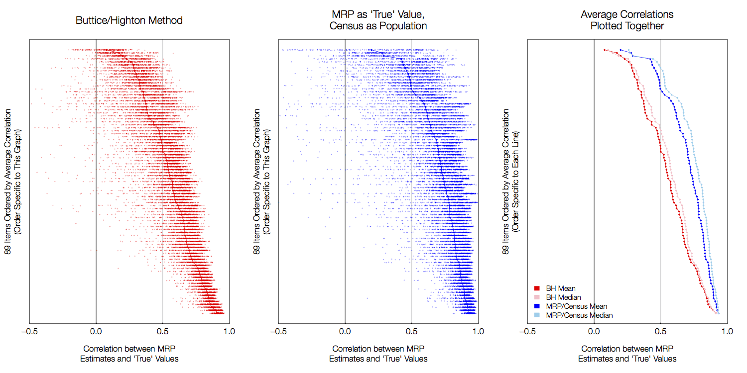
An alternative approach could (a) define the “true value” using MRP from the full data, and (b) use the census as the population dataset from which to post-stratify. Because BH made their replication data available, it was fairly easy to do just that. The following figure shows the results (click for full-size version):

The left-hand plot replicates BH’s Figure 1 (other figures can be similarly replicated). Each row of the figure is for one of the 89 policy items. For each item, each dot represents the correlation between the “true value” and one of the 200 samples drawn for each item (jittered to better show the distribution). The line indicates the average correlation for each item. The rows are ordered by this average correlation.

The middle plot shows the same results using the alternative method — I am using MRP on the full dataset as the “true value”, and using census population data to poststratify. It is immediately apparent that the correlations are substantially higher under this formulation.

Because of the jittering, we can also see (in both graphs) that the highest mass of dots is substantially to the right of the average line! The average correlations appear to be “dragged down” by a few outliers with very small correlations. An alternative measure, then, is to examine the median correlation instead of the mean. This is done in the right-hand plot, where we see that the median values are substantially higher than the means.

(It is worth noting that each line is ordered by its value — the top row has the lowest average correlation under each measure, but that means that the rows are not comparable across graphs. This, does, however, allow us to clearly see the “low-to-high” curve for both methods.)

Some might consider setting the “true value” using full MRP to be tipping the scales in favor of MRP. But because state is included as a term in the model, this can at worst be considered equivalent to weighting the survey responses by the terms in the model (which is helpful in and of itself, as BH’s “true values” do not account for sample weights).

In addition to the described alternative procedure, LP suggest a number of methods to adjust BH’s correlations to account for this noise, writing “if one wants to take the BH paper as showing what a random application of MRP can do, without inspecting the response model to confirm that it is working sufficiently well, our best guess is that the correlation to the desired true state levels is about a third higher than BH report.”

Although the method above is quite different than what LP describe, the average correlations are indeed about 40% higher than those reported by BH, on average.

With all that said, I am in agreement with some of the basic principles suggested by BH and expanded upon by LP — it is important to be careful using MRP! Results are indeed variable — though, in my view, not nearly as variable as found by BH.

For my part, I’m thrilled that MRP is becoming a mainstream tool, and I think it’s great that people are following the work of Lax and Phillips and trying to understand what is needed to make MRP work most effectively.